9 Scikit-Learn for Machine Learning

Machine learning (ML) is a field of artificial intelligence that enables systems to learn and improve from experience without being explicitly programmed. It involves the use of algorithms and statistical models to analyze and draw inferences from patterns in data. Scikit-learn is one of the most popular and robust machine learning libraries in Python, designed for ease of use, flexibility, and performance.

Caution

This chapter provides Python code for using ML tools for regression, classification and clustering. While supporting text is provided to explain the context of the techniques, use of the contents of this chapter for research or development is strongly discouraged unless the reader has taken a dedicated course on ML.
The code is provided for educational purposes only. It is important to note that the code provided here is not optimized for production use. For production use, it is recommended to use the appropriate libraries and tools that are optimized for performance, scalability, and security.

What is Scikit-Learn?

Scikit-learn is an open-source Python library that provides simple and efficient tools for data mining and data analysis. Built on top of NumPy, SciPy, and matplotlib, it offers a wide range of supervised and unsupervised learning algorithms through a consistent interface in Python. It is well-suited for a variety of tasks, including classification, regression, clustering, and dimensionality reduction.

Key Features

Simple and Efficient Tools: Scikit-learn offers a variety of tools for data preprocessing, model selection, and evaluation, making it easy to implement and compare different machine learning models.
Wide Range of Algorithms: It includes implementations of many machine learning algorithms such as support vector machines, random forests, gradient boosting, k-means, and more.
Integration with Other Libraries: Seamlessly integrates with other scientific and numerical libraries in Python, such as NumPy, SciPy, and pandas.
Extensive Documentation: Provides comprehensive documentation and a wealth of tutorials, examples, and user guides to help users get started and deepen their understanding of machine learning concepts.

Why Use Scikit-Learn?

Scikit-learn is widely used in academia and industry due to its simplicity, performance, and extensive range of functionalities. It allows researchers and practitioners to focus on the problem at hand without worrying about the underlying implementation details. Moreover, its consistent API design and extensive documentation make it a great tool for both beginners and experienced machine learning practitioners.

Supervised learning

Supervised learning is a type of machine learning where the algorithm is trained on labeled data, meaning input data paired with the correct output. The aim is to learn a function that maps inputs to outputs based on these examples. During training, the algorithm learns patterns and relationships between input features and their corresponding outputs, enabling it to predict outputs for new, unseen data. Supervised learning has two main categories: classification and regression. Classification predicts discrete output variables or class labels, such as determining if an email is spam. Regression predicts continuous output variables, such as estimating house prices based on features like location and size. Widely used in applications like image recognition, speech recognition, natural language processing, and predictive analytics, supervised learning is a powerful tool for making predictions and identifying data patterns.

The ML Model

In case you have a dataset (maybe scarce) containing input and output data and you want to find a relationship between them, possibly for prediction purposes, we need a model. The model can be physical, i.e. based on fundamental physical principles that simulate the actual process that generates the data or data-driven i.e. purely based based on measurements. Ofter development of a physical model is not feasible or rather not required to understand the relationship between the input and output data points. In that case we can use statistical non-linear regression to develop a model purely based on the input and output measurement data.

9.1 Regression

Regression is a fundamental concept in machine learning and statistics, primarily used for predicting continuous outcomes. It involves modeling the relationship between a dependent variable (often called the target or output) and one or more independent variables (called features or predictors). The goal of regression is to find a function that best describes the relationship between the input and output data, allowing us to make predictions on new, unseen data points.

import numpy as np
#%matplotlib inline
import matplotlib.pyplot as plt

9.1.1 True Physics

Let us assume that we have the true physical description of the process that relates the input and output data described by a certain function. Usually we do not have this. Here, we are using this just to find out how much far we are from the model that is predicted from just a few observations !

# define the true physical process and draw some data
input_start = -1
input_end   = 5

input_true = np.linspace(start=input_start, stop=input_end, num=1000).reshape(-1, 1)
input_true.shape

(1000, 1)

output_true = np.squeeze(input_true * np.sin(input_true)*np.cos(input_true)*np.tan(input_true))

output_true.shape

(1000,)

plt.figure(figsize=(3, 3))
plt.plot(input_true, output_true, label='True Physics', linestyle="-", color='black')
plt.legend()
plt.xlabel('input')
plt.ylabel('output')
plt.title('True Physics')

Text(0.5, 1.0, 'True Physics')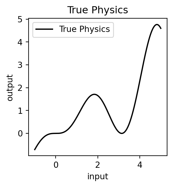

The generated true physics is quite complex. It is also strongly non-linear ! Now let us simulate the process of making experiments to generate outputs for a selected few inputs.

9.1.2 Experimental measurements

available_measurements = 10

Let us randomly extract 6 points from the true physical process. This is like performing 10 experiments at different locations. Right now these are random.

rng = np.random.RandomState(0)
measurement_indices = rng.choice(np.arange(input_true.size), size=available_measurements, replace=False)
measurement_indices

array([993, 859, 298, 553, 672, 971,  27, 231, 306, 706])

Add gaussian noise with a given standard deviation

noise_std = 0.15

input_measurement = input_true[measurement_indices]
output_measurement = output_true[measurement_indices] 
input_measurement, output_measurement

(array([[ 4.96396396],
        [ 4.15915916],
        [ 0.78978979],
        [ 2.32132132],
        [ 3.03603604],
        [ 4.83183183],
        [-0.83783784],
        [ 0.38738739],
        [ 0.83783784],
        [ 3.24024024]]),
 array([ 4.65636706,  3.01087732,  0.39836331,  1.24154687,  0.03370267,
         4.76322524, -0.46277436,  0.05528432,  0.46277436,  0.03142975]))

output_measurement = output_measurement + rng.normal(loc=0.0, scale=noise_std, size=output_measurement.shape)

output_measurement

array([ 4.72151009,  3.09471209,  0.52477185,  1.45049338,  0.08883534,
        4.47835002, -0.6925601 ,  0.06668465,  0.38367645,  0.00822619])

plt.errorbar(input_measurement, output_measurement, noise_std, linestyle='None', color='tab:red', marker='.', 
             markersize=10,label='Measurements')


plt.legend()
plt.xlabel('input')
plt.ylabel('output')
plt.title('Measurements')

Text(0.5, 1.0, 'Measurements')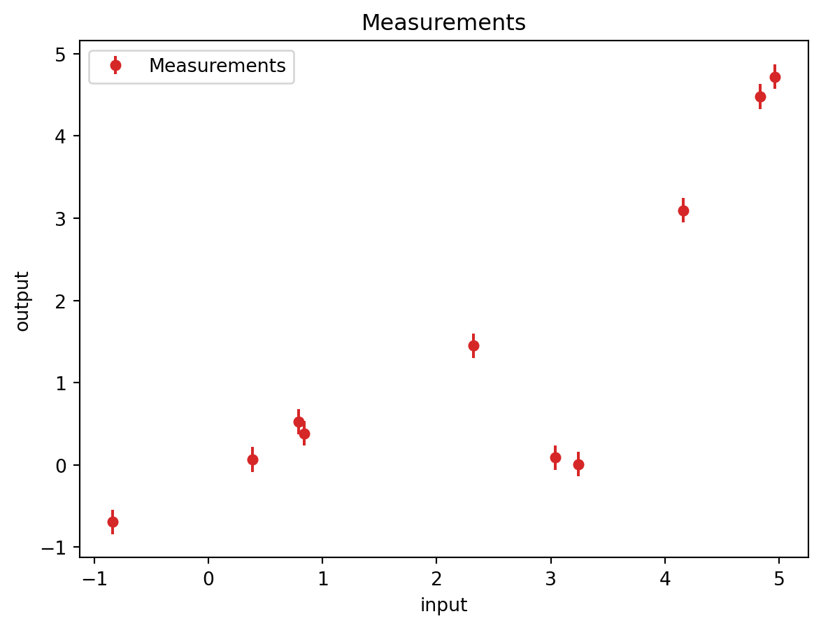

CHALLENGE: Using just the above experimental measurements, try to predict the true physics using machine learning!

9.1.3 Kernel Ridge Regression

Kernel Ridge Regression (KRR) is a versatile and powerful regression technique that combines the advantages of ridge regression and kernel methods. It extends the linear ridge regression model by mapping the input features into a higher-dimensional space using a kernel function, which allows it to capture complex, non-linear relationships between the input variables and the target variable. The kernel function, such as the Gaussian (RBF), polynomial, or linear kernel, plays a crucial role in transforming the data and enabling the model to perform well on a wide range of problems. By incorporating a regularization term in the objective function, KRR mitigates overfitting and enhances the model’s generalization capabilities. This makes it particularly useful in scenarios where the relationship between the predictors and the response variable is highly non-linear, and the risk of overfitting is significant.

from sklearn.gaussian_process.kernels import RBF
kernel = 1 * RBF(length_scale=1.0, length_scale_bounds=(1e-2, 1e2))

output_measurement

array([ 4.72151009,  3.09471209,  0.52477185,  1.45049338,  0.08883534,
        4.47835002, -0.6925601 ,  0.06668465,  0.38367645,  0.00822619])

from sklearn.kernel_ridge import KernelRidge
krr = KernelRidge(kernel = kernel, alpha=noise_std**2)

krr.fit(input_measurement, output_measurement)

KernelRidge(alpha=0.0225, kernel=1**2 * RBF(length_scale=1))

In a Jupyter environment, please rerun this cell to show the HTML representation or trust the notebook.
On GitHub, the HTML representation is unable to render, please try loading this page with nbviewer.org.

Make predictions

new_input_measurements = np.linspace(input_start, input_end, 20).reshape(-1, 1)
new_input_measurements

array([[-1.        ],
       [-0.68421053],
       [-0.36842105],
       [-0.05263158],
       [ 0.26315789],
       [ 0.57894737],
       [ 0.89473684],
       [ 1.21052632],
       [ 1.52631579],
       [ 1.84210526],
       [ 2.15789474],
       [ 2.47368421],
       [ 2.78947368],
       [ 3.10526316],
       [ 3.42105263],
       [ 3.73684211],
       [ 4.05263158],
       [ 4.36842105],
       [ 4.68421053],
       [ 5.        ]])

output_krr_prediction = krr.predict(new_input_measurements)
output_krr_prediction

array([-0.70798005, -0.61099339, -0.45894208, -0.28280242, -0.07891206,
        0.19921947,  0.59910269,  1.09662668,  1.55288221,  1.75860386,
        1.56486146,  1.01988242,  0.40230558,  0.10014448,  0.39719416,
        1.30458386,  2.54799936,  3.71159639,  4.43808167,  4.56633603])

# Plot the results
plt.figure()
plt.errorbar(input_measurement, output_measurement, noise_std, linestyle='None', color='tab:red', marker='.', 
             markersize=10,label='Measurements')
plt.scatter(new_input_measurements, output_krr_prediction, color='green', label='Prediction')
plt.plot(input_true, output_true, label='True Physics', linestyle="-", color='black')
plt.xlabel('input')
plt.ylabel('output')
plt.title('Kernel Ridge Regression')
plt.legend()
plt.show()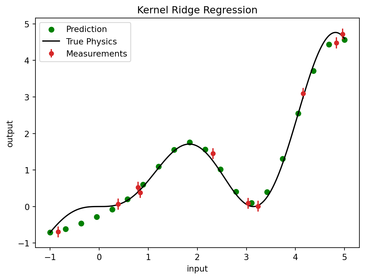

9.1.4 Gaussian Process Regression

Gaussian Process Regression (GPR) is a non-parametric, Bayesian approach to regression that provides a flexible and powerful framework for modeling complex data. Unlike traditional parametric models, GPR does not assume a fixed form for the underlying function, instead, it defines a distribution over possible functions directly. This is achieved through the use of a Gaussian process, which is a collection of random variables, any finite number of which have a joint Gaussian distribution. A key component of GPR is the kernel function, which determines the covariance structure of the data and allows the model to capture intricate patterns and correlations. By integrating out the parameters, GPR naturally incorporates uncertainty in the predictions, offering not only point estimates but also a measure of confidence in these predictions. This probabilistic nature makes GPR particularly well-suited for applications where quantifying uncertainty is important, such as in Bayesian optimization, time-series forecasting, and spatial data analysis. The flexibility and robustness of GPR make it an essential tool for tackling complex regression tasks in various scientific and engineering domains.

from sklearn.gaussian_process import GaussianProcessRegressor

#help(GaussianProcessRegressor)
gaussian_process = GaussianProcessRegressor(kernel=kernel, alpha=noise_std**2, n_restarts_optimizer=9)
gaussian_process.fit(input_measurement, output_measurement)

GaussianProcessRegressor(alpha=0.0225, kernel=1**2 * RBF(length_scale=1),
                         n_restarts_optimizer=9)

Make predictions

new_input_measurements = np.linspace(input_start, input_end, 50).reshape(-1, 1)
gpr_mean_prediction, gpr_std_prediction = gaussian_process.predict(new_input_measurements, return_std=True)

plt.plot(input_true, output_true, label='True Physics', linestyle='-', color='black')
plt.errorbar(input_measurement, output_measurement, noise_std, linestyle='None', color='tab:red', marker='.', 
             markersize=10,label="Observations")

plt.scatter(new_input_measurements, gpr_mean_prediction, label='Mean prediction', color='green')

plt.fill_between(
    new_input_measurements.ravel(),
    gpr_mean_prediction - 1.96 * gpr_std_prediction,
    gpr_mean_prediction + 1.96 * gpr_std_prediction,
    color='tab:green',
    alpha=0.5,
    label=r'95% confidence interval',)

plt.legend()
plt.xlabel('$input$')
plt.ylabel('$output$')
plt.title('Measurements and Model predictions')
plt.show()

9.1.5 Decision Tree Regression

Decision Tree Regression is a non-linear regression technique that models the relationship between input features and a continuous target variable through a tree-like structure of decisions. This method involves recursively partitioning the feature space into distinct and non-overlapping regions by making binary decisions at each node of the tree. Each split is chosen to maximize the homogeneity of the target variable within the resulting regions, typically using criteria such as mean squared error reduction. The final prediction is made by averaging the target variable within each region, corresponding to the leaf nodes of the tree. Decision Tree Regression is highly interpretable, as the hierarchical structure of the tree can be easily visualized and understood. It is capable of capturing complex interactions between features without requiring any specific assumptions about the underlying data distribution. However, decision trees can be prone to overfitting, especially when the tree grows too deep, which can be mitigated through techniques like pruning or by using ensemble methods such as Random Forests or Gradient Boosting. This makes Decision Tree Regression a versatile and powerful tool for various regression tasks, particularly when interpretability and the ability to model non-linear relationships are crucial.

from sklearn.tree import DecisionTreeRegressor

# Fit regression model
dtr_1 = DecisionTreeRegressor(max_depth=2)
dtr_2 = DecisionTreeRegressor(max_depth=5)
dtr_3 = DecisionTreeRegressor(max_depth=7)

dtr_1.fit(input_measurement, output_measurement)
dtr_2.fit(input_measurement, output_measurement)
dtr_3.fit(input_measurement, output_measurement)

DecisionTreeRegressor(max_depth=7)

Make predictions

new_input_measurements = np.linspace(input_start, input_end, 50).reshape(-1, 1)

dtr_prediction_1 = dtr_1.predict(new_input_measurements)
dtr_prediction_2 = dtr_2.predict(new_input_measurements)
dtr_prediction_3 = dtr_3.predict(new_input_measurements)

# Plot the results
plt.figure()
#plt.plot(input_true, output_true, label='True Physics', linestyle="-", color='black')
plt.errorbar(input_measurement, output_measurement, noise_std, linestyle='None', color='tab:red', marker='.', 
             markersize=10,label='Measurements')
plt.plot(new_input_measurements, dtr_prediction_1, color='orange', label='max_depth=2', linewidth=2, linestyle=':')
plt.plot(new_input_measurements, dtr_prediction_2, color='blue', label='max_depth=5', linewidth=2, linestyle='-.')
plt.plot(new_input_measurements, dtr_prediction_3, color='green', label='max_depth=7', linewidth=2, linestyle='--')
plt.xlabel('input')
plt.ylabel('output')
plt.title('Decision Tree Regression')
plt.legend()
plt.show()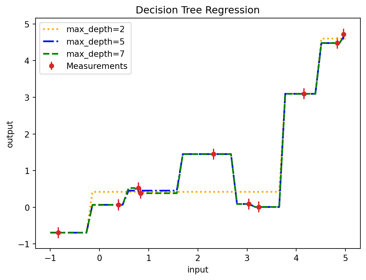

9.2 Classification

There are many different classification methods available for classifying datasets. Here are a few examples:

Logistic Regression: A statistical model that predicts the probability of an event occurring, given a set of independent variables.
Decision Tree: A tree-like model of decisions and their possible consequences, used to classify data by assigning them to one of several categories.
Random Forest: An ensemble method that combines multiple decision trees to improve classification accuracy.
Support Vector Machines (SVM): A type of supervised learning algorithm that can be used for classification, regression, and outlier detection.
Naive Bayes: A probabilistic classifier based on Bayes’ theorem that assumes independence between features.
k-Nearest Neighbors (k-NN): A non-parametric algorithm that classifies data points based on the k closest training examples in the feature space.
Neural Networks: A machine learning model inspired by the structure and function of the human brain, consisting of interconnected nodes that process information and produce output.

# import libraries
import numpy as np
from sklearn.datasets import make_classification
from sklearn.model_selection import train_test_split
from sklearn.linear_model import LogisticRegression
from sklearn.tree import DecisionTreeClassifier
from sklearn.ensemble import RandomForestClassifier
from sklearn.svm import SVC
from sklearn.naive_bayes import GaussianNB
from sklearn.neighbors import KNeighborsClassifier
from sklearn.neural_network import MLPClassifier
from sklearn.metrics import accuracy_score

# generate toy dataset
X, y = make_classification(n_samples=1000, n_features=10, n_informative=5, n_classes=3, random_state=42)

array([[-2.56891645, -0.25740861, -2.67935708, ..., -1.21337007,
        -1.47310497, -0.84638564],
       [ 0.62286056,  0.53454361,  0.01828302, ..., -1.09353229,
        -0.46979071, -0.18802193],
       [-0.17125115, -0.49627753,  1.61334708, ...,  0.71453069,
         3.47599878,  0.6233862 ],
       ...,
       [ 1.49733849, -1.14885141, -0.78734187, ..., -0.99204356,
         0.71868115, -0.45139203],
       [-0.17397319,  0.16781324,  2.60761116, ..., -0.2693521 ,
         0.65157292, -0.31914351],
       [-1.58610983,  0.89359204, -1.30742057, ..., -0.05661209,
        -0.54079228, -1.0986882 ]])

array([1, 1, 0, 1, 0, 0, 2, 2, 1, 2, 0, 0, 1, 1, 0, 2, 1, 1, 0, 1, 0, 1,
       1, 2, 0, 1, 2, 1, 2, 0, 2, 0, 0, 1, 0, 1, 2, 2, 0, 1, 1, 2, 0, 0,
       1, 0, 2, 0, 1, 2, 2, 0, 0, 2, 0, 2, 2, 2, 2, 0, 1, 0, 0, 0, 2, 2,
       0, 2, 2, 1, 0, 2, 2, 0, 2, 2, 2, 2, 0, 1, 0, 0, 2, 2, 0, 0, 1, 0,
       2, 2, 0, 0, 0, 2, 0, 2, 2, 2, 0, 1, 1, 2, 2, 1, 0, 0, 2, 0, 1, 1,
       2, 0, 1, 2, 0, 2, 1, 1, 0, 0, 1, 1, 1, 0, 2, 1, 1, 2, 0, 2, 0, 1,
       2, 0, 0, 0, 2, 0, 1, 2, 0, 2, 2, 2, 2, 0, 1, 0, 2, 2, 1, 1, 2, 1,
       1, 0, 0, 1, 0, 1, 2, 2, 0, 0, 1, 2, 0, 2, 2, 1, 1, 1, 2, 1, 1, 1,
       1, 1, 0, 2, 1, 2, 0, 0, 0, 0, 1, 1, 0, 2, 2, 0, 0, 0, 1, 0, 0, 2,
       0, 2, 2, 0, 1, 0, 1, 2, 2, 2, 1, 0, 1, 1, 2, 2, 1, 1, 0, 2, 1, 2,
       0, 2, 1, 0, 2, 2, 0, 1, 0, 0, 2, 0, 1, 1, 1, 2, 0, 1, 0, 2, 1, 2,
       1, 0, 0, 2, 2, 2, 1, 2, 0, 1, 0, 0, 2, 2, 1, 2, 0, 2, 2, 1, 0, 0,
       0, 2, 2, 1, 0, 2, 1, 1, 2, 2, 1, 0, 2, 2, 0, 0, 2, 1, 2, 0, 2, 0,
       2, 0, 0, 2, 2, 0, 2, 0, 0, 0, 2, 2, 1, 0, 0, 2, 0, 0, 0, 2, 2, 2,
       1, 1, 1, 2, 0, 0, 2, 1, 2, 1, 1, 2, 0, 2, 1, 2, 2, 0, 1, 2, 2, 1,
       2, 2, 0, 1, 2, 2, 2, 1, 2, 2, 2, 1, 1, 0, 2, 0, 0, 2, 2, 1, 0, 2,
       1, 2, 2, 2, 0, 0, 1, 0, 1, 1, 2, 2, 1, 1, 0, 0, 2, 1, 1, 1, 2, 0,
       2, 1, 1, 1, 0, 1, 1, 2, 1, 2, 1, 0, 1, 2, 2, 0, 1, 0, 0, 0, 1, 0,
       2, 0, 2, 2, 1, 2, 1, 2, 0, 1, 2, 2, 2, 1, 0, 1, 0, 2, 1, 1, 0, 0,
       1, 1, 0, 2, 2, 2, 2, 0, 2, 2, 2, 1, 0, 2, 1, 1, 2, 0, 1, 0, 0, 2,
       2, 2, 1, 1, 1, 0, 1, 1, 2, 1, 0, 0, 1, 2, 1, 2, 2, 0, 0, 1, 1, 0,
       1, 0, 2, 1, 2, 1, 0, 0, 2, 1, 0, 2, 2, 0, 2, 2, 1, 1, 0, 1, 2, 1,
       2, 1, 2, 0, 0, 1, 2, 0, 1, 0, 2, 1, 0, 0, 2, 1, 1, 1, 1, 0, 0, 2,
       0, 1, 0, 0, 0, 1, 2, 2, 0, 2, 0, 0, 2, 0, 0, 2, 1, 2, 0, 0, 1, 1,
       1, 0, 0, 2, 1, 2, 1, 1, 2, 1, 1, 1, 2, 0, 2, 1, 1, 1, 1, 1, 1, 0,
       2, 2, 2, 0, 1, 1, 1, 2, 0, 2, 0, 2, 0, 2, 2, 0, 2, 0, 0, 2, 2, 2,
       1, 2, 0, 2, 1, 2, 0, 1, 0, 2, 0, 1, 0, 1, 0, 2, 2, 2, 2, 0, 2, 1,
       1, 0, 2, 1, 1, 1, 2, 0, 0, 0, 1, 2, 2, 2, 0, 0, 2, 0, 1, 2, 1, 2,
       2, 1, 0, 0, 0, 2, 1, 1, 0, 0, 2, 0, 1, 1, 0, 0, 0, 2, 2, 1, 1, 1,
       1, 1, 2, 2, 0, 2, 2, 0, 1, 1, 0, 2, 1, 0, 0, 2, 2, 0, 0, 0, 1, 2,
       1, 2, 0, 0, 1, 0, 2, 1, 1, 0, 2, 2, 1, 2, 1, 2, 0, 1, 1, 0, 0, 2,
       1, 1, 1, 2, 0, 2, 0, 2, 2, 0, 2, 2, 1, 0, 0, 0, 1, 0, 0, 1, 2, 2,
       2, 2, 0, 0, 2, 0, 2, 2, 0, 2, 2, 1, 1, 2, 0, 0, 1, 0, 1, 1, 1, 1,
       1, 0, 1, 1, 2, 1, 2, 1, 0, 0, 2, 2, 2, 1, 1, 1, 0, 2, 2, 1, 0, 1,
       1, 0, 1, 0, 0, 1, 1, 0, 0, 0, 2, 1, 1, 2, 2, 1, 0, 2, 0, 1, 1, 1,
       0, 1, 2, 0, 0, 0, 1, 0, 1, 2, 1, 1, 2, 1, 1, 0, 1, 2, 0, 0, 2, 1,
       2, 0, 2, 1, 0, 0, 0, 0, 2, 1, 0, 1, 0, 1, 1, 0, 1, 0, 1, 1, 0, 2,
       0, 0, 0, 2, 2, 2, 2, 1, 0, 1, 2, 0, 1, 0, 0, 0, 2, 2, 1, 0, 2, 2,
       2, 1, 2, 1, 1, 1, 0, 1, 2, 2, 0, 0, 1, 1, 1, 1, 1, 2, 1, 1, 0, 1,
       1, 1, 0, 1, 1, 0, 0, 2, 1, 2, 2, 2, 2, 2, 2, 1, 1, 2, 2, 1, 2, 0,
       0, 1, 2, 2, 0, 1, 1, 1, 1, 1, 1, 0, 0, 1, 1, 0, 2, 0, 1, 0, 0, 0,
       2, 1, 2, 0, 2, 2, 1, 1, 0, 0, 1, 2, 0, 2, 1, 2, 0, 0, 1, 1, 1, 2,
       2, 1, 1, 1, 0, 0, 0, 0, 2, 1, 2, 1, 1, 1, 0, 0, 0, 2, 1, 1, 0, 0,
       0, 2, 0, 1, 0, 1, 1, 2, 1, 0, 0, 2, 1, 0, 2, 2, 2, 0, 0, 2, 0, 2,
       2, 1, 1, 0, 0, 1, 1, 1, 2, 0, 0, 2, 2, 0, 1, 2, 2, 0, 1, 0, 1, 1,
       1, 2, 1, 1, 1, 2, 1, 0, 0, 1])

# split dataset into training and testing sets
X_train, X_test, y_train, y_test = train_test_split(X, y, test_size=0.3, random_state=42)

# initialize models
models = {
    'Logistic Reg': LogisticRegression(random_state=42),
    'Decision Tree': DecisionTreeClassifier(random_state=42),
    'Random Forest': RandomForestClassifier(random_state=42),
    'SVM': SVC(random_state=42),
    'Naive Bayes': GaussianNB(),
    'k-NN': KNeighborsClassifier(),
    'Neural Network': MLPClassifier(random_state=42)
}

# fit and evaluate models
results = {}
for name, model in models.items():
    model.fit(X_train, y_train)
    y_pred = model.predict(X_test)
    accuracy = accuracy_score(y_test, y_pred)
    results[name] = accuracy

/Users/jt_official/anaconda3/lib/python3.11/site-packages/sklearn/neural_network/_multilayer_perceptron.py:691: ConvergenceWarning:

Stochastic Optimizer: Maximum iterations (200) reached and the optimization hasn't converged yet.

results

{'Logistic Reg': 0.72,
 'Decision Tree': 0.7766666666666666,
 'Random Forest': 0.86,
 'SVM': 0.86,
 'Naive Bayes': 0.7666666666666667,
 'k-NN': 0.8433333333333334,
 'Neural Network': 0.8666666666666667}

9.3 Unsupervised Learning

Unsupervised learning is a type of machine learning where the algorithm is trained on unlabeled data. Unlike supervised learning, unsupervised learning doesn’t have a predefined target variable, which means that the algorithm tries to find patterns and relationships in the data without any explicit guidance.

The goal of unsupervised learning is to identify hidden structures or groupings in the data, which can help in data exploration and feature extraction. Unsupervised learning algorithms work by clustering similar data points together, based on the underlying structure or distribution of the data.

One popular unsupervised learning algorithm is k-means clustering, which involves dividing a dataset into k clusters, based on the similarity of their features. Another example is principal component analysis (PCA), which is used to reduce the dimensionality of high-dimensional data by finding the most important features that explain the majority of the variation in the data.

Unsupervised learning has several advantages, including the ability to discover hidden patterns and relationships in the data, without the need for explicit labels or target variables. It can also help in feature selection and data compression, which can be useful for reducing the computational complexity of machine learning algorithms.

Unsupervised learning is widely used in many applications, including image segmentation, anomaly detection, and market segmentation. It is a powerful technique for exploring and understanding complex datasets, without the need for human supervision or guidance.

9.3.1 Clustering

There are many methods for clustering using Python, here are some of the most popular ones:

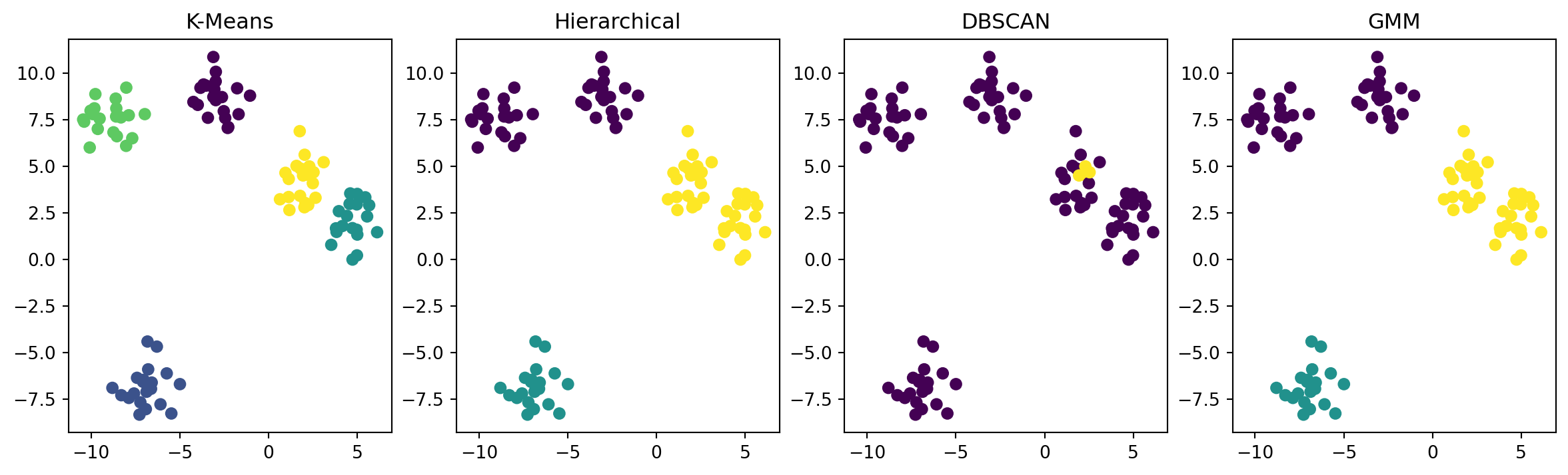
K-Means Clustering: It is a popular unsupervised machine learning algorithm that partitions data points into K clusters based on similarity. The K-Means algorithm aims to minimize the sum of squared distances between data points and their respective cluster centers. The Scikit-learn library provides an implementation of K-Means clustering in Python.
Hierarchical Clustering: This algorithm builds a hierarchy of clusters by either merging smaller clusters into larger ones (agglomerative) or splitting larger clusters into smaller ones (divisive). The hierarchy can be represented as a tree-like diagram called a dendrogram. The Scikit-learn library provides an implementation of hierarchical clustering in Python.
DBSCAN Clustering: This algorithm groups together points that are closely packed together while leaving out points that are far away from the clusters. The algorithm does not require specifying the number of clusters beforehand, and it can handle noisy data. The Scikit-learn library provides an implementation of DBSCAN clustering in Python.
Gaussian Mixture Model (GMM) Clustering: This algorithm models the probability distribution of the data using a mixture of Gaussian distributions. The algorithm determines the optimal number of clusters and their parameters by maximizing the likelihood of the data. The Scikit-learn library provides an implementation of GMM clustering in Python.

import numpy as np
import matplotlib.pyplot as plt
from sklearn.datasets import make_blobs
from sklearn.cluster import KMeans, AgglomerativeClustering, DBSCAN
from sklearn.mixture import GaussianMixture

# Generate a toy dataset with 100 data points and 5 clusters
X, y = make_blobs(n_samples=100, centers=5, random_state=42)

array([[ -6.2927701 ,  -4.68965397],
       [  2.03530213,   5.61498563],
       [ -2.97261532,   8.54855637],
       [  0.64463087,   3.22362652],
       [ -8.73867639,   6.82004726],
       [ -7.22234171,  -7.68238686],
       [  5.00151486,   1.32804993],
       [  4.1607046 ,   1.78751071],
       [  4.6040528 ,   3.53781334],
       [ -3.10983631,   8.72259238],
       [ -3.6601912 ,   9.38998415],
       [ -6.87451373,  -7.11469673],
       [  1.17550652,   2.64660433],
       [ -2.62484591,   8.71318243],
       [  5.45240466,   3.32940971],
       [ -8.31638619,   7.62050759],
       [  1.57578528,   5.01785035],
       [  0.95140774,   4.64392397],
       [ -7.40938739,  -6.36684216],
       [ -6.97255325,   7.79735584],
       [ -7.87495163,   7.73630384],
       [  6.11777288,   1.45489947],
       [ -2.26723535,   7.10100588],
       [ -5.73680438,  -6.12817656],
       [ -9.81300943,   8.11060752],
       [ -7.67973218,   6.5028406 ],
       [  2.08050895,   3.01848126],
       [  1.13278581,   3.34564127],
       [  2.19548116,   4.54676894],
       [  4.98349713,   0.21012953],
       [ -4.99344129,  -6.70553178],
       [ -8.61086782,   8.63066567],
       [  1.77691212,   3.40771539],
       [  1.1384428 ,   4.31517666],
       [  2.02013373,   2.79507219],
       [ -8.54525528,   6.6091715 ],
       [ -2.97867201,   9.55684617],
       [ -3.11090424,  10.86656431],
       [ -3.05358035,   9.12520872],
       [  3.96295684,   2.58484597],
       [ -7.58168029,  -7.20777174],
       [  4.42020695,   2.33028226],
       [  4.97114227,   2.94871481],
       [  3.53354386,   0.77696306],
       [ -8.57844496,   8.10534579],
       [ -1.77073104,   9.18565441],
       [ -3.98771961,   8.29444192],
       [ -6.91433896,  -8.04878763],
       [ -8.58783491,   7.66997112],
       [  3.10535148,   5.21525361],
       [  1.79883745,   4.87545205],
       [  5.55528095,   2.30192079],
       [  4.7269259 ,   1.67416233],
       [ -8.29499793,  -7.30075492],
       [  4.56786871,   2.97670258],
       [ -9.51835248,   7.55577661],
       [  2.29899103,   4.9886348 ],
       [  2.23639398,   2.91571278],
       [ -3.4172217 ,   7.60198243],
       [ -4.23411546,   8.4519986 ],
       [  3.83138523,   1.47141264],
       [ -3.52202874,   9.32853346],
       [ -9.75775199,   8.87345732],
       [ -7.27173534,  -8.34362454],
       [-10.44581099,   7.50815677],
       [ -6.81939698,  -4.41686748],
       [  2.49553786,   4.08862264],
       [  2.3800876 ,   4.72223608],
       [ -7.07198816,  -6.57856225],
       [  1.7576434 ,   6.88162072],
       [-10.07527847,   6.0030663 ],
       [ -6.78254964,  -5.9114646 ],
       [ -8.79839841,  -6.90662347],
       [ -7.0409129 ,  -6.47605874],
       [  2.64796758,   3.304294  ],
       [ -8.0162676 ,   9.2203159 ],
       [  4.96396281,   1.5880874 ],
       [-10.38899119,   7.39208589],
       [  1.94519853,   4.50260353],
       [ -5.47683288,  -8.28196066],
       [  2.5373355 ,   4.67523751],
       [ -6.6220768 ,  -6.95455551],
       [ -9.90063147,   7.79711535],
       [  5.00127444,   3.51120625],
       [ -8.02481054,   6.0926586 ],
       [ -2.30033403,   7.054616  ],
       [-10.02963125,   7.98007652],
       [ -1.68665271,   7.79344248],
       [ -3.83738367,   9.21114736],
       [ -2.44166942,   7.58953794],
       [ -9.62158105,   7.0014614 ],
       [ -2.96983639,  10.07140835],
       [ -6.58350691,  -6.61905432],
       [  4.73163961,  -0.01439923],
       [ -6.08859524,  -7.78949705],
       [ -1.04354885,   8.78850983],
       [ -7.87016352,  -7.44640732],
       [ -2.52269485,   7.9565752 ],
       [  5.67087836,   2.9044498 ],
       [  3.80066131,   1.66395731]])

array([2, 4, 0, 4, 3, 2, 1, 1, 1, 0, 0, 2, 4, 0, 1, 3, 4, 4, 2, 3, 3, 1,
       0, 2, 3, 3, 4, 4, 4, 1, 2, 3, 4, 4, 1, 3, 0, 0, 0, 1, 2, 1, 1, 1,
       3, 0, 0, 2, 3, 4, 4, 1, 1, 2, 1, 3, 4, 4, 0, 0, 1, 0, 3, 2, 3, 2,
       4, 4, 2, 4, 3, 2, 2, 2, 4, 3, 1, 3, 4, 2, 4, 2, 3, 1, 3, 0, 3, 0,
       0, 0, 3, 0, 2, 1, 2, 0, 2, 0, 1, 1])

# Perform K-Means clustering
kmeans = KMeans(n_clusters=5, random_state=42)
kmeans_labels = kmeans.fit_predict(X)

# Perform Hierarchical clustering
hierarchical = AgglomerativeClustering(n_clusters=3)
hierarchical_labels = hierarchical.fit_predict(X)

# Perform DBSCAN clustering
dbscan = DBSCAN(eps=0.5, min_samples=5)
dbscan_labels = dbscan.fit_predict(X)

# Perform GMM clustering
gmm = GaussianMixture(n_components=3)
gmm_labels = gmm.fit_predict(X)

/Users/jt_official/anaconda3/lib/python3.11/site-packages/sklearn/cluster/_kmeans.py:1412: FutureWarning:

The default value of `n_init` will change from 10 to 'auto' in 1.4. Set the value of `n_init` explicitly to suppress the warning

kmeans_labels

array([1, 4, 0, 4, 3, 1, 2, 2, 2, 0, 0, 1, 4, 0, 2, 3, 4, 4, 1, 3, 3, 2,
       0, 1, 3, 3, 4, 4, 4, 2, 1, 3, 4, 4, 4, 3, 0, 0, 0, 2, 1, 2, 2, 2,
       3, 0, 0, 1, 3, 4, 4, 2, 2, 1, 2, 3, 4, 4, 0, 0, 2, 0, 3, 1, 3, 1,
       4, 4, 1, 4, 3, 1, 1, 1, 4, 3, 2, 3, 4, 1, 4, 1, 3, 2, 3, 0, 3, 0,
       0, 0, 3, 0, 1, 2, 1, 0, 1, 0, 2, 2], dtype=int32)

# Plot the clustering results
plt.figure(figsize=(15, 4))
plt.subplot(141)
plt.scatter(X[:, 0], X[:, 1], c=kmeans_labels)
plt.title('K-Means')
plt.subplot(142)
plt.scatter(X[:, 0], X[:, 1], c=hierarchical_labels)
plt.title('Hierarchical')
plt.subplot(143)
plt.scatter(X[:, 0], X[:, 1], c=dbscan_labels)
plt.title('DBSCAN')
plt.subplot(144)
plt.scatter(X[:, 0], X[:, 1], c=gmm_labels)
plt.title('GMM')
plt.show()