8 Scientific Python (SciPy)

Scipy is a powerful open-source scientific computing library for the Python programming language. It was created in 2001 by Travis Oliphant, a computational scientist, and over the years, it has grown to become one of the most widely used libraries in the scientific and engineering communities.

Scipy provides a wide range of modules for tasks such as numerical integration, optimization, signal processing, linear algebra, and more. It is built on top of the NumPy library, which provides support for arrays and matrices. The combination of Scipy and NumPy creates a powerful toolset for scientific computing in Python.

The library is continuously maintained and updated by a team of developers, and it is widely used in academia, research, and industry. Its primary goal is to provide efficient and easy-to-use tools for scientific computing and data analysis.

Some of the key applications of Scipy include machine learning, image processing, signal processing, optimization, and simulation. It is also commonly used in fields such as physics, chemistry, biology, and engineering.

Overall, Scipy has become an essential tool for anyone working in scientific computing and data analysis in Python, and its continued development and innovation make it an exciting library to work with.

8.1 Integration

Numerical evaluation of a function of the type

\(\displaystyle \int_a^b \int_a^b f(x, y) dxdy\)

can be performed using numerical quadrature. In SciPy, for e.g. the quad function and dblquad among others, can be used for 1 variable and double integration respectively. Multiple variable integration is also available.

from scipy.integrate import quad

# define a simple function for the integrand
def f_1d(x, a, b):
    """
    implements a simple quadratic function, with intercept at zero
    """
    return (a**b)*x**2

x_lower = 0 # the lower limit of x
x_upper = 1 # the upper limit of x

val, abserr = quad(f_1d, x_lower, x_upper, args=(1, 2))
print(val, abserr)

0.3333333333333333 3.700743415417188e-15

8.2 Ordinary differential equations (ODEs)

SciPy is often used to solve ODEs and system of coupled ODEs ! The odeint function is used to solve ODEs.

8.2.1 Lotka-Volterra Equations

Let’s solve a simple 2D system of ordinary differential equations (ODEs) and plot the results. We’ll use the solve_ivp function from SciPy’s integrate module.

Consider the following system of ODEs:

\[ \frac{dx}{dt} = f(x, y) \] \[ \frac{dy}{dt} = g(x, y) \]

where \(x\) and \(y\) are the dependent variables, and \(f(x, y)\) and \(g(x, y)\) are functions that describe the rates of change of \(x\) and \(y\) with respect to time \(t\).

For this example, let’s use the Lotka-Volterra equations (predator-prey model):

\[ \frac{dx}{dt} = \alpha x - \beta xy \] \[ \frac{dy}{dt} = \delta xy - \gamma y \]

where \(\alpha\), \(\beta\), \(\gamma\), and \(\delta\) are constants.

Here’s the Python code to solve this system and plot the results:

import numpy as np
import matplotlib.pyplot as plt
from scipy.integrate import solve_ivp

# Define the Lotka-Volterra equations
def lotka_volterra(t, z, alpha, beta, delta, gamma):
    x, y = z
    dxdt = alpha * x - beta * x * y
    dydt = delta * x * y - gamma * y
    return [dxdt, dydt]

# Parameters
alpha = 1.0
beta = 0.1
delta = 0.075
gamma = 1.5

# Initial conditions: [prey population, predator population]
z0 = [10, 5]

# Time span
t_span = (0, 10)
t_eval = np.linspace(*t_span, 1000)

# Solve the system of ODEs
solution = solve_ivp(lotka_volterra, t_span, z0, args=(alpha, beta, delta, gamma), t_eval=t_eval)

# Extract the results
t = solution.t
x = solution.y[0]
y = solution.y[1]

# Plot the results
fig, ax = plt.subplots(figsize=(6, 6))

# Plot prey population
ax.plot(t, x, label='Prey (x)', color='blue')

# Plot predator population
ax.plot(t, y, label='Predator (y)', color='red')

# Add labels and legend
ax.set_xlabel('Time')
ax.set_ylabel('Population')
ax.legend()
ax.grid()

plt.show()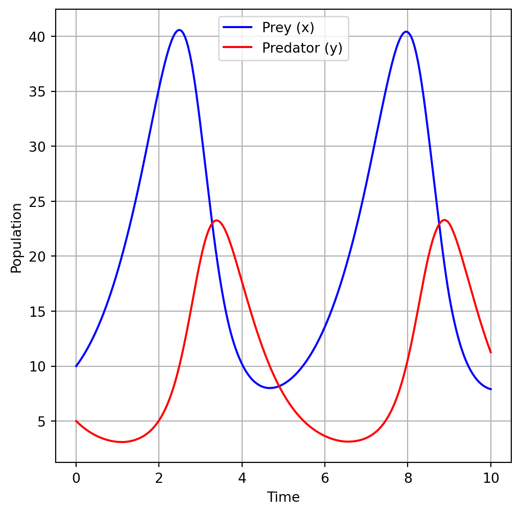

Running this code will produce a plot showing the dynamics of the prey and predator populations over time according to the Lotka-Volterra model.

8.2.2 Modelling Infection and recovery

At rate \(\beta\), when a susceptible meets an infected, two infected persons exist. \(S + I \rightarrow 2 I\) At rate \(\gamma\) the infected recovers ! \(I \rightarrow R\)

	R1	R2
S	-1	0
I	+1	-1
R	0	1

Let us consider a simple epidemiological model that simulates the infection and recovery of a population ! The ordinary differential equations describing this is given by:

\[\begin{aligned} & \frac{dS}{dt} = - \beta I S, \\ & \frac{dI}{dt} = \beta I S- \gamma I, \\ & \frac{dR}{dt} = \gamma I, \end{aligned}\]

from scipy.integrate import odeint

beta = 0.01
gamma = 0.5


def dx(x, t):
    """
    The right-hand side of the model
    """
    S = x[0]
    I = x[1]
    R = x[2]
    
    
    dS = -beta*I*S*t
    dI = beta*I*S -gamma*I
    dR = gamma*I
    
    return [dS, dI, dR]

# choose an initial state
x0 = [90, 10, 0]

# time coodinate to solve the ODE for: from 0 to 10 days
t = np.linspace(0, 20, 350)

# solve the ODE problem
x = odeint(dx, x0, t)

import matplotlib.pyplot as plt

fig, axes = plt.subplots(figsize=(6, 6))
axes.plot(t, x[:, 0], 'r', label='Susceptible')
axes.plot(t, x[:, 1], 'b', label="Infected")
axes.plot(t, x[:, 2], 'g', label="Recovered")
axes.legend()
axes.set_xlabel('days')
axes.set_ylabel('Number')
plt.show()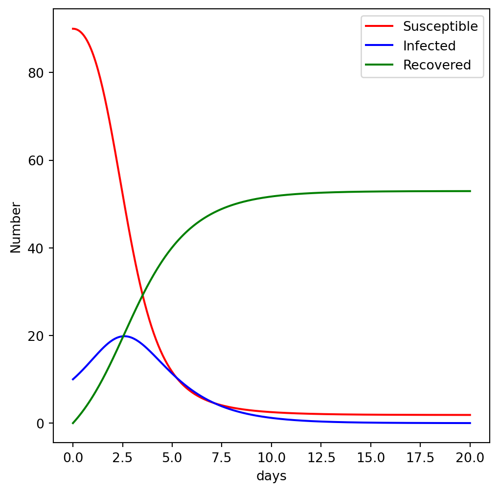

8.3 Optimization

Let us look at a few very simple cases of optimization. For a more detailed introduction to optimization with SciPy see: http://scipy-lectures.github.com/advanced/mathematical_optimization/index.html

from scipy import optimize

8.3.1 Finding a minima of a 1D function

Let’s first look at how to find the minima of a simple function of a single variable:

def f(x):
    """
    a function that returns the square of the input data
    """
    return x**2

fig, ax  = plt.subplots()
x = np.linspace(-5, 3, 100)
ax.plot(x, f(x));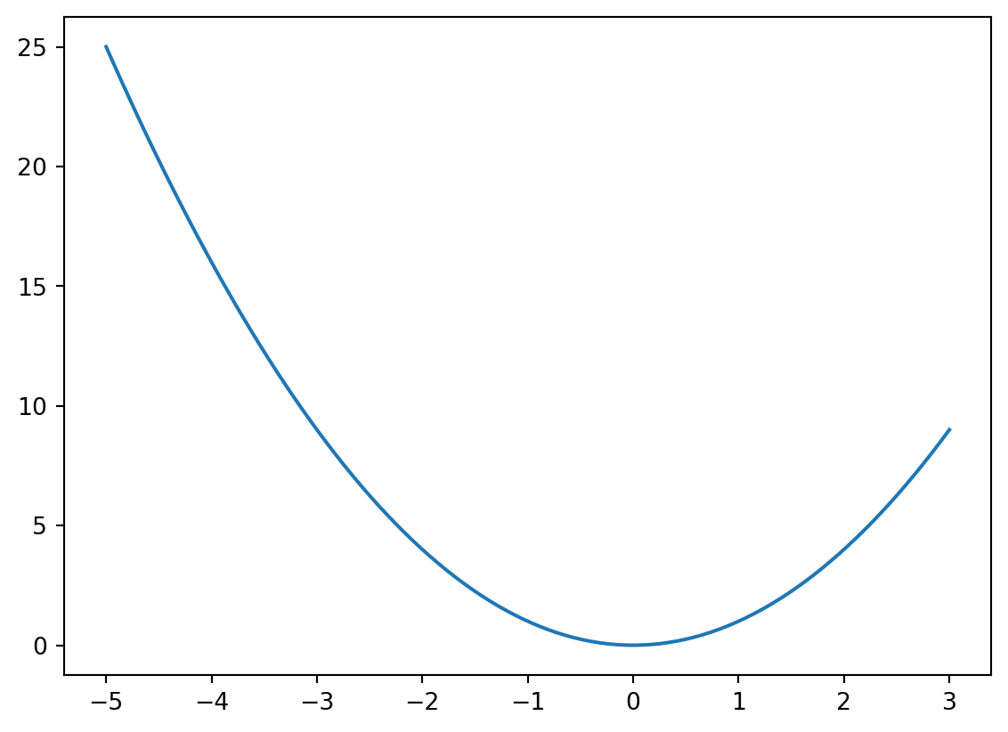

We can use the fmin_bfgs function to find the minima of a function:

x_min = optimize.fmin_bfgs(f, -2)
x_min

Optimization terminated successfully.
         Current function value: 0.000000
         Iterations: 2
         Function evaluations: 6
         Gradient evaluations: 3

array([-1.79994222e-08])

optimize.fmin_bfgs(f, -5)

Optimization terminated successfully.
         Current function value: 0.000000
         Iterations: 3
         Function evaluations: 8
         Gradient evaluations: 4

array([-2.54405594e-08])

We can also use the brent or fminbound functions. They have a bit different syntax and use different algorithms.

8.3.2 Optimization of a 2D function

Let’s consider a common 2D objective function, the Rosenbrock function, which is often used to test optimization algorithms. The function is defined as:

\[f(x, y) = (a - x)^2 + b(y - x^2)^2 \]

where \(a\) and \(b\) are constants. For our example, let’s set \(a = 1\) and \(b = 100\).

We’ll use SciPy’s optimization capabilities to find the minimum of this function and create a contour plot with contour labels.

import numpy as np
import matplotlib.pyplot as plt
from scipy.optimize import minimize

# Define the Rosenbrock function
def rosenbrock(x):
    a = 1
    b = 100
    return (a - x[0])**2 + b * (x[1] - x[0]**2)**2

# Perform the optimization
initial_guess = [0, 0]
result = minimize(rosenbrock, initial_guess, method='BFGS')
opt_x, opt_y = result.x

# Generate a grid of points
x = np.linspace(-2, 2, 400)
y = np.linspace(-1, 3, 400)
X, Y = np.meshgrid(x, y)
Z = (1 - X)**2 + 100 * (Y - X**2)**2


# Plot the contour
fig, ax = plt.subplots(figsize=(7, 7))
contour = ax.contour(X, Y, Z, levels=np.logspace(-1, 3, 20), cmap='viridis')
ax.clabel(contour, inline=True, fontsize=8)
ax.plot(opt_x, opt_y, 'r*', markersize=10, label='Optimum')
ax.set_xlabel('x')
ax.set_ylabel('y')
ax.legend()
#plt.colorbar()
plt.show()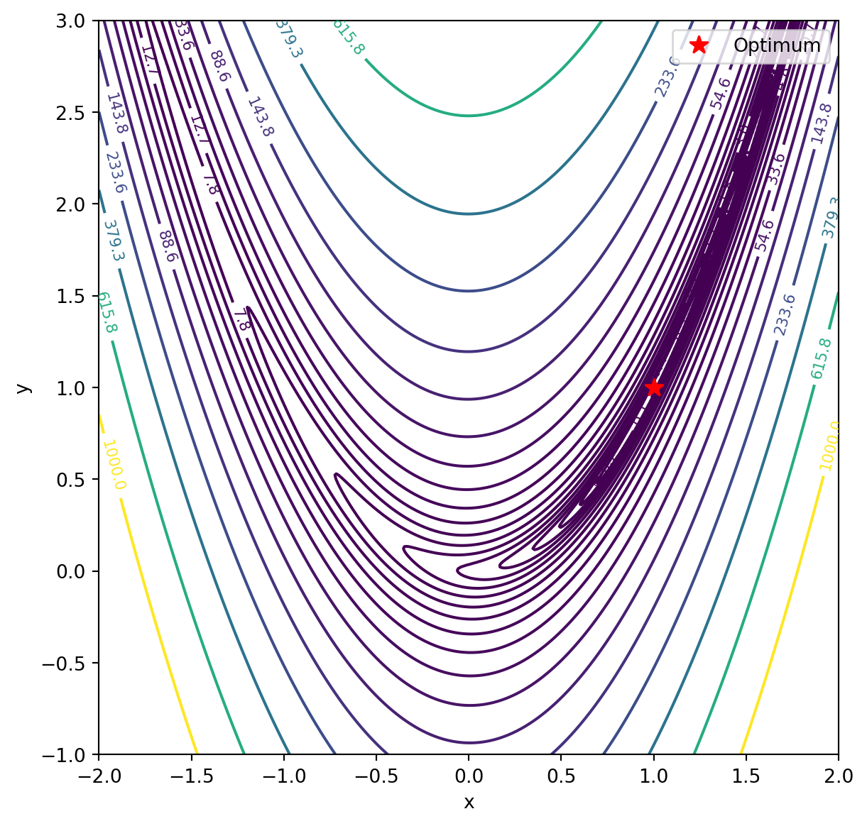

8.4 Further reading

Here are some of the most frequently used functions from the SciPy library:

scipy.integrate.quad: Computes a definite integral of a function from a to b using Gaussian quadrature.

scipy.optimize.minimize: Finds the minimum of a function using various optimization algorithms.

scipy.stats.norm: Provides functions for working with normal (Gaussian) distributions, including PDF, CDF, and random number generation.

scipy.linalg.eig: Computes the eigenvalues and eigenvectors of a square matrix.

scipy.signal.convolve: Computes the convolution of two signals.

scipy.fft.fft: Computes the one-dimensional discrete Fourier Transform.

scipy.special.gamma: Computes the gamma function and related functions.

scipy.interpolate.interp1d: Interpolates a one-dimensional function.

scipy.spatial.distance.pdist: Computes pairwise distances between observations in a dataset.

scipy.cluster.hierarchy.linkage: Computes hierarchical clusters from a distance matrix.