5  Arrays and Array Operations using NumPy

NumPy was first released in 2006 as an open-source extension to the Python programming language that provided support for large, multi-dimensional arrays and matrices, as well as a large library of mathematical functions to operate on those arrays. NumPy was created by Travis Oliphant, who was inspired by MATLAB and the desire to provide a similar set of capabilities in Python. Since its initial release, NumPy has become an integral part of the scientific Python ecosystem and is widely used in data analysis, machine learning, and scientific computing.

# Generate random data
import numpy as np
import matplotlib.pyplot as plt
data = np.random.rand(50, 50)  # 50 samples, 50 features

# Compute the covariance matrix
cov_matrix = np.cov(data, rowvar=False)

# Compute eigenvalues and eigenvectors
eigenvalues, eigenvectors = np.linalg.eig(cov_matrix)
transformed_data = np.dot(data, eigenvectors)
# Create subplots
fig, axes = plt.subplots(4, 1, figsize=(6, 24))

# Plot the original data
axes[0].imshow(data, cmap='Spectral', aspect='auto', interpolation='none')
axes[0].set_title('Data Matrix')
axes[0].set_xlabel('Feature Index')
axes[0].set_ylabel('Data Point Index')

# Plot the covariance matrix
axes[1].imshow(cov_matrix, cmap='Spectral', aspect='auto', interpolation='none')
axes[1].set_title('Covariance Matrix')
axes[1].set_xlabel('Feature Index')
axes[1].set_ylabel('Feature Index')

# Plot the eigenvectors
axes[2].imshow(eigenvectors, cmap='Spectral', aspect='auto', interpolation='none')
axes[2].set_title('Eigenvectors Matrix')
axes[2].set_xlabel('Eigenvector Index')
axes[2].set_ylabel('Feature Index')

# Plot the transformed data
axes[3].imshow(transformed_data, cmap='Spectral', aspect='auto', interpolation='none')
axes[3].set_title('Transformed Data (PCA)')
axes[3].set_xlabel('Principal Component Index')
axes[3].set_ylabel('Data Point Index')

plt.tight_layout()
plt.show()

Data, Covariance and Eigenvectors

In the above example, a datset with 50 data points with 50 features is subjected to principal component analysis using numpy. This procedure performs a dimensional reduction that can be used to extract the most relevant features.

To use numpy you need to import the module, using for example:

import numpy as np # alias

In the numpy package the terminology used for the mathematical quantities vectors, matrices and higher-dimensional data sets is array.

There are a number of ways to create new numpy arrays, for example from

1. a List or a Tuple
2. using generator functions in numpy such as arange, linspace, etc.
3. reading data from files

5.1 Generating an Array from lists and tuples

For example, to create new vector and matrix arrays from Python lists we can use the numpy.array function.

l = [1, 2, 3, 4] # list mutable
t = (1, 2, 3, 4) # tuple immutable

v = np.array(l) # Numpy Array using l or t

v

array([1, 2, 3, 4])

Consider the following matrix, a two dimensional data structure. Where data is related by thier positions in a two dimensional grid !

\[ \begin{bmatrix} 1 & 2 & 3 \\ 2 & 4 & 5 \\ 3 & 5 & 6 \end{bmatrix} \]

l_2d = [[1.0, 2, 3], [2, 4, 5], [3, 5, 6]]

M = np.array(l_2d)

M

array([[1., 2., 3.],
       [2., 4., 5.],
       [3., 5., 6.]])

The v and M belong to the ndarray type as you can find out from the following test !

type(v), type(M)

(numpy.ndarray, numpy.ndarray)

We can get the shape of an array by using the ndarray.shape property.

M.shape

(3, 3)

The number of elements in the array is available through the ndarray.size property:

M.size

9

Equivalently, we could use the function numpy.shape and numpy.size

np.shape(M)

(3, 3)

np.size(M)

9

Note:

The package name is required if the variable is passed to the function. Using the dot notation, the function already knows the data type !

What is the benefit of using NumPy instead of using Python lists ?

• Lists and Tuples can contain any kind of object but in contrast the Numpy arrays are homogeneous and all items in a numpy array are of the same type and hence creation, manipulation of Numpy arrays etc. are efficient

Using the numpy specific attribute dtype (data type), we can see what type the data of an array is:

M.dtype

dtype('float64')

If we update a value inside the array as a floating point, the value will be reverted to an integer version.

print(np.pi)

3.141592653589793

M[1, 1] = np.pi
M

array([[1.        , 2.        , 3.        ],
       [2.        , 3.14159265, 5.        ],
       [3.        , 5.        , 6.        ]])

If we try to introduce a string type, the operation fails. Thus in contrast to a Python list, Numpy arrays are homogeneous ! We can also explicitly define the type of the array data when we create it, using the dtype keyword argument:

M = np.array(l_2d, dtype=complex)

M

array([[1.+0.j, 2.+0.j, 3.+0.j],
       [2.+0.j, 4.+0.j, 5.+0.j],
       [3.+0.j, 5.+0.j, 6.+0.j]])

Common data types that can be used with dtype are: int, float, complex, bool, object, etc. Specifying the datatype can save memory ! Here is the list of numeric data types and the associated memory footprint !

Numpy data type	Storage Size	Description
np.bool_	1 byte	can hold boolean values, like (True or False) or (0 or 1)
np.byte	1 byte	can hold values from 0 to 255
np.ubyte	1 byte	can hold values from -128 to 127
np.short	2 bytes	can hold values from -32,768 to 32,767
np.ushort	2 bytes	can hold values from 0 to 65,535
np.uintc	2 or 4 bytes	can hold values from 0 to 65,535 or 0 to 4,294,967,295
np.int_	8 bytes	can hold values from -9223372036854775808 to 9223372036854775807
np.uint	8 bytes	0 to 18446744073709551615
np.longlong	8 bytes	can hold values from -9223372036854775808 to 9223372036854775807
np.ulonglong	8 bytes	0 to 18446744073709551615
np.half / np.float16		allows half float precision with Format: sign bit, 5 bits exponent, 10 bits mantissa
np.single	4 bytes	allows single float precision Format: sign bit, 8 bits exponent, 23 bits mantissa
np.double	8 bytes	allows double float precision Format: sign bit, 11 bits exponent, 52 bits mantissa.
np.longdouble	8 bytes	extension of float
np.csingle	8 bytes	can hold complex with real and imaginary parts up to single-precision float
np.cdouble	16 bytes	can hold complex with real and imaginary parts up to double-precision float
np.clongdouble	16 bytes	extension of float for complex number
np.int8	1 byte	can hold values from -128 to 127
np.int16	2 bytes	can hold values from -32,768 to 32,767
np.int32	4 bytes	can hold values from -2,147,483,648 to 2,147,483,647
np.int64	8 bytes	can hold values from -9223372036854775808 to 9223372036854775807
np.uint8	1 byte	can hold values from 0 to 255
np.uint16	2 bytes	can hold values from 0 to 65,535
np.uint32	4 bytes	can hold values from 0 to 4,294,967,295
np.uint64	8 bytes	can hold values from 0 to 18446744073709551615
np.intp	4 bytes	a signed integer used for indexing
np.uintp	4 bytes	an unsigned integer used for holding a pointer
np.float32	4 bytes	single float precision
np.float64	8 bytes	double float precision
np.complex64	8 bytes	single float precision in complex numbers
np.complex128	16 bytes	double float precision in complex numbers

import sys
print('Size of the Matrix Array is '+ str(sys.getsizeof(M)) + ' bytes')

Size of the Matrix Array is 272 bytes

5.2 4.2 Creating an Array using array-generating functions

For larger arrays it is impractical to initialize the data manually, using explicit python lists. Instead we can use one of the many functions in numpy that generate arrays of different forms. Some of the more common are:

5.2.1 4.2.1 arange

# create a range of data starting at 0 and ending at(15-1) and incremented by 1

x = np.arange(0, 15, 1) # arguments: start, stop, step 

x

array([ 0,  1,  2,  3,  4,  5,  6,  7,  8,  9, 10, 11, 12, 13, 14])

Also floating point values can be generated. Let us create a list of real numbers. Let the list be some x.

x = np.arange(-1, 1.1, 0.1)

x

array([-1.00000000e+00, -9.00000000e-01, -8.00000000e-01, -7.00000000e-01,
       -6.00000000e-01, -5.00000000e-01, -4.00000000e-01, -3.00000000e-01,
       -2.00000000e-01, -1.00000000e-01, -2.22044605e-16,  1.00000000e-01,
        2.00000000e-01,  3.00000000e-01,  4.00000000e-01,  5.00000000e-01,
        6.00000000e-01,  7.00000000e-01,  8.00000000e-01,  9.00000000e-01,
        1.00000000e+00])

Having defined x, we can then generate functions using the inbuilt numpy function library of mathematical functions !

https://numpy.org/doc/stable/reference/routines.math.html

\(f(x) = x^4\)

We can make plots using the matplotlib.pyplot library and using the the syntax as given below ! Commands that start with % in Jupyter are specific to the Jupyter notebook. Here we use the matplotlib inline to tell Jupyter to plot the images in this notebook !

%matplotlib inline 
import matplotlib.pyplot as plt

x

array([-1.00000000e+00, -9.00000000e-01, -8.00000000e-01, -7.00000000e-01,
       -6.00000000e-01, -5.00000000e-01, -4.00000000e-01, -3.00000000e-01,
       -2.00000000e-01, -1.00000000e-01, -2.22044605e-16,  1.00000000e-01,
        2.00000000e-01,  3.00000000e-01,  4.00000000e-01,  5.00000000e-01,
        6.00000000e-01,  7.00000000e-01,  8.00000000e-01,  9.00000000e-01,
        1.00000000e+00])

x**4

array([1.00000000e+00, 6.56100000e-01, 4.09600000e-01, 2.40100000e-01,
       1.29600000e-01, 6.25000000e-02, 2.56000000e-02, 8.10000000e-03,
       1.60000000e-03, 1.00000000e-04, 2.43086534e-63, 1.00000000e-04,
       1.60000000e-03, 8.10000000e-03, 2.56000000e-02, 6.25000000e-02,
       1.29600000e-01, 2.40100000e-01, 4.09600000e-01, 6.56100000e-01,
       1.00000000e+00])

plt.plot(x, x**4)

5.2.2 linspace

Using linspace (linear space) we can generate a specified number of data points within a given range. The range end points are also included.

np.linspace(0, 10, 50) # start, end, number of items

array([ 0.        ,  0.20408163,  0.40816327,  0.6122449 ,  0.81632653,
        1.02040816,  1.2244898 ,  1.42857143,  1.63265306,  1.83673469,
        2.04081633,  2.24489796,  2.44897959,  2.65306122,  2.85714286,
        3.06122449,  3.26530612,  3.46938776,  3.67346939,  3.87755102,
        4.08163265,  4.28571429,  4.48979592,  4.69387755,  4.89795918,
        5.10204082,  5.30612245,  5.51020408,  5.71428571,  5.91836735,
        6.12244898,  6.32653061,  6.53061224,  6.73469388,  6.93877551,
        7.14285714,  7.34693878,  7.55102041,  7.75510204,  7.95918367,
        8.16326531,  8.36734694,  8.57142857,  8.7755102 ,  8.97959184,
        9.18367347,  9.3877551 ,  9.59183673,  9.79591837, 10.        ])

5.2.3 logspace

Using logspace we can generate logarithmically spaced points !

\[ base^{start} \rightarrow base^{end}\]

lgspace = np.logspace(0, 10, 10, base=2) # start, end, number of items, base

lgspace

array([1.00000000e+00, 2.16011948e+00, 4.66611616e+00, 1.00793684e+01,
       2.17726400e+01, 4.70315038e+01, 1.01593667e+02, 2.19454460e+02,
       4.74047853e+02, 1.02400000e+03])

plt.plot(lgspace)
plt.show()

5.2.4 mgrid

Similar to creating a one dimensional data (series data), two dimensional data can also be generated !

x, y = np.mgrid[0:3, 0:3] # similar to the arange. : is used to demarcate the ranges. 

x

array([[0, 0, 0],
       [1, 1, 1],
       [2, 2, 2]])

y

array([[0, 1, 2],
       [0, 1, 2],
       [0, 1, 2]])

5.2.5 random data

we can also generate an array with random data ! The function random.rand

https://numpy.org/doc/stable/reference/random/index.html

# uniform random numbers in [0, 1]
np.random.rand(3, 3)

array([[0.80425808, 0.91644266, 0.47945464],
       [0.21569627, 0.52090131, 0.89417937],
       [0.50636599, 0.67670055, 0.51481776]])

# standard normal distributed random numbers
np.random.randn(3, 3)

array([[-1.27736451e+00,  1.59161186e+00, -3.15222576e-01],
       [-1.63659815e+00, -1.11057424e+00,  1.58779671e+00],
       [-1.30381795e-03, -9.16393344e-01,  1.31435067e+00]])

We can visualize 2D arrays using imshow.

np.random.randn(10, 10)

array([[-1.67515109, -1.93245625,  1.2615826 ,  0.69348647, -0.16594454,
         1.44398401, -0.53415791,  0.64797016,  0.828767  ,  0.01751825],
       [-0.3638571 , -0.75646745, -1.66850663,  0.03083016, -0.25965105,
         2.13601146,  0.52458306,  1.16150728, -0.35282144,  1.07374027],
       [ 0.14522132, -1.22808633, -0.63322584, -0.35155261, -0.48921836,
        -0.0268312 , -0.76753532,  0.75151109,  0.70637612, -1.67628368],
       [-0.11671744, -0.68997496, -1.30395157, -1.73608655, -0.0801369 ,
        -0.35752284,  1.49908668,  0.35738585, -1.30701492,  1.70858813],
       [ 1.74885291,  0.48121687,  0.32328458, -0.71135126,  0.53170209,
         1.59452732, -0.92616407, -0.05157693, -1.237883  , -0.71519852],
       [-0.08348287,  0.39636936, -1.3645921 ,  0.54865215, -0.61140374,
        -0.62733116,  0.35739261, -0.53088816,  0.17516257, -0.06341533],
       [-0.6983727 ,  1.70713101,  0.23749051, -0.52713372, -0.88230791,
         1.68793038, -0.06480881, -0.43290539,  0.37201036, -0.41139954],
       [-1.52896209,  0.30351605, -0.81867851, -1.1193333 , -0.54335377,
        -0.21380058,  1.64256138, -1.14491203,  0.01830303, -0.78131983],
       [ 0.80107231,  0.99466504, -0.20027495,  1.29342589,  1.70677514,
         0.79313249,  0.50654972, -1.72837271,  0.81041233,  0.20362425],
       [ 1.5826136 , -0.89964506, -0.83235601, -1.07621675,  0.75140168,
        -0.0852246 ,  0.04652429,  0.80063524, -0.99034519, -1.15093594]])

plt.imshow(np.random.randn(100, 100))
plt.show()

5.2.6 zeros and ones

np.zeros((3, 3))

array([[0., 0., 0.],
       [0., 0., 0.],
       [0., 0., 0.]])

np.ones((3, 3))

array([[1., 1., 1.],
       [1., 1., 1.],
       [1., 1., 1.]])

5.3 Importing and Exporting files

5.3.1 Comma-separated values (CSV)

Ofter after processing data, we want to save them. They can be saved as a common CSV or the python internal npy format.

Using np.savetxt we can store a Numpy array to a file in CSV format:

M = np.random.rand(100, 100)

M

array([[0.17067143, 0.3826854 , 0.03930981, ..., 0.36198335, 0.49802238,
        0.12879821],
       [0.21299847, 0.2190781 , 0.53682624, ..., 0.65250561, 0.48938648,
        0.58293481],
       [0.22215091, 0.50411751, 0.36649375, ..., 0.90346575, 0.76319889,
        0.40866292],
       ...,
       [0.97625385, 0.36392632, 0.73232771, ..., 0.19198673, 0.52626557,
        0.79145138],
       [0.92992187, 0.13624226, 0.53239969, ..., 0.76426326, 0.9714768 ,
        0.63239779],
       [0.5189122 , 0.05317721, 0.32686314, ..., 0.55126585, 0.88348397,
        0.11199564]])

Let us first create a string with the absolute location of the folder !

folder = './data/'

np.savetxt(folder + 'random_array_100x100.csv', M)

If the file is stored in the same folder as that of this Jupyter Notebook, then just the filename demarcated by apostrophes are sufficient.

imported_array = np.loadtxt(folder + 'random_array_100x100.csv')

imported_array

array([[0.17067143, 0.3826854 , 0.03930981, ..., 0.36198335, 0.49802238,
        0.12879821],
       [0.21299847, 0.2190781 , 0.53682624, ..., 0.65250561, 0.48938648,
        0.58293481],
       [0.22215091, 0.50411751, 0.36649375, ..., 0.90346575, 0.76319889,
        0.40866292],
       ...,
       [0.97625385, 0.36392632, 0.73232771, ..., 0.19198673, 0.52626557,
        0.79145138],
       [0.92992187, 0.13624226, 0.53239969, ..., 0.76426326, 0.9714768 ,
        0.63239779],
       [0.5189122 , 0.05317721, 0.32686314, ..., 0.55126585, 0.88348397,
        0.11199564]])

5.3.2 Numpy’s native file format

In case the data will be processed only within the python framework then use the functions numpy.save and numpy.load:

np.save(folder + 'random_array.npy', M)

np.load(folder + 'random_array.npy')

array([[0.17067143, 0.3826854 , 0.03930981, ..., 0.36198335, 0.49802238,
        0.12879821],
       [0.21299847, 0.2190781 , 0.53682624, ..., 0.65250561, 0.48938648,
        0.58293481],
       [0.22215091, 0.50411751, 0.36649375, ..., 0.90346575, 0.76319889,
        0.40866292],
       ...,
       [0.97625385, 0.36392632, 0.73232771, ..., 0.19198673, 0.52626557,
        0.79145138],
       [0.92992187, 0.13624226, 0.53239969, ..., 0.76426326, 0.9714768 ,
        0.63239779],
       [0.5189122 , 0.05317721, 0.32686314, ..., 0.55126585, 0.88348397,
        0.11199564]])

%matplotlib inline
import matplotlib.pyplot as plt # Alias

import numpy as np

5.4 Importing an external csv file

folder = './data/'

temperature_anomaly = np.loadtxt(folder + 't_ano.csv')

temperature_anomaly

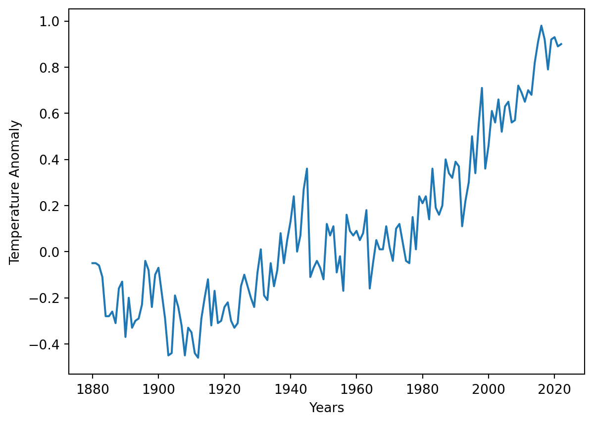
array([[ 1.880e+03, -5.000e-02],
       [ 1.881e+03, -5.000e-02],
       [ 1.882e+03, -6.000e-02],
       [ 1.883e+03, -1.100e-01],
       [ 1.884e+03, -2.800e-01],
       [ 1.885e+03, -2.800e-01],
       [ 1.886e+03, -2.600e-01],
       [ 1.887e+03, -3.100e-01],
       [ 1.888e+03, -1.600e-01],
       [ 1.889e+03, -1.300e-01],
       [ 1.890e+03, -3.700e-01],
       [ 1.891e+03, -2.000e-01],
       [ 1.892e+03, -3.300e-01],
       [ 1.893e+03, -3.000e-01],
       [ 1.894e+03, -2.900e-01],
       [ 1.895e+03, -2.300e-01],
       [ 1.896e+03, -4.000e-02],
       [ 1.897e+03, -8.000e-02],
       [ 1.898e+03, -2.400e-01],
       [ 1.899e+03, -1.000e-01],
       [ 1.900e+03, -7.000e-02],
       [ 1.901e+03, -1.800e-01],
       [ 1.902e+03, -2.900e-01],
       [ 1.903e+03, -4.500e-01],
       [ 1.904e+03, -4.400e-01],
       [ 1.905e+03, -1.900e-01],
       [ 1.906e+03, -2.400e-01],
       [ 1.907e+03, -3.200e-01],
       [ 1.908e+03, -4.500e-01],
       [ 1.909e+03, -3.300e-01],
       [ 1.910e+03, -3.500e-01],
       [ 1.911e+03, -4.400e-01],
       [ 1.912e+03, -4.600e-01],
       [ 1.913e+03, -2.900e-01],
       [ 1.914e+03, -2.000e-01],
       [ 1.915e+03, -1.200e-01],
       [ 1.916e+03, -3.200e-01],
       [ 1.917e+03, -1.700e-01],
       [ 1.918e+03, -3.100e-01],
       [ 1.919e+03, -3.000e-01],
       [ 1.920e+03, -2.400e-01],
       [ 1.921e+03, -2.200e-01],
       [ 1.922e+03, -3.000e-01],
       [ 1.923e+03, -3.300e-01],
       [ 1.924e+03, -3.100e-01],
       [ 1.925e+03, -1.500e-01],
       [ 1.926e+03, -1.000e-01],
       [ 1.927e+03, -1.500e-01],
       [ 1.928e+03, -2.000e-01],
       [ 1.929e+03, -2.400e-01],
       [ 1.930e+03, -9.000e-02],
       [ 1.931e+03,  1.000e-02],
       [ 1.932e+03, -1.900e-01],
       [ 1.933e+03, -2.100e-01],
       [ 1.934e+03, -5.000e-02],
       [ 1.935e+03, -1.500e-01],
       [ 1.936e+03, -8.000e-02],
       [ 1.937e+03,  8.000e-02],
       [ 1.938e+03, -5.000e-02],
       [ 1.939e+03,  5.000e-02],
       [ 1.940e+03,  1.300e-01],
       [ 1.941e+03,  2.400e-01],
       [ 1.942e+03,  0.000e+00],
       [ 1.943e+03,  7.000e-02],
       [ 1.944e+03,  2.700e-01],
       [ 1.945e+03,  3.600e-01],
       [ 1.946e+03, -1.100e-01],
       [ 1.947e+03, -7.000e-02],
       [ 1.948e+03, -4.000e-02],
       [ 1.949e+03, -7.000e-02],
       [ 1.950e+03, -1.200e-01],
       [ 1.951e+03,  1.200e-01],
       [ 1.952e+03,  7.000e-02],
       [ 1.953e+03,  1.100e-01],
       [ 1.954e+03, -9.000e-02],
       [ 1.955e+03, -2.000e-02],
       [ 1.956e+03, -1.700e-01],
       [ 1.957e+03,  1.600e-01],
       [ 1.958e+03,  9.000e-02],
       [ 1.959e+03,  7.000e-02],
       [ 1.960e+03,  9.000e-02],
       [ 1.961e+03,  5.000e-02],
       [ 1.962e+03,  8.000e-02],
       [ 1.963e+03,  1.800e-01],
       [ 1.964e+03, -1.600e-01],
       [ 1.965e+03, -5.000e-02],
       [ 1.966e+03,  5.000e-02],
       [ 1.967e+03,  1.000e-02],
       [ 1.968e+03,  1.000e-02],
       [ 1.969e+03,  1.100e-01],
       [ 1.970e+03,  2.000e-02],
       [ 1.971e+03, -4.000e-02],
       [ 1.972e+03,  1.000e-01],
       [ 1.973e+03,  1.200e-01],
       [ 1.974e+03,  4.000e-02],
       [ 1.975e+03, -4.000e-02],
       [ 1.976e+03, -5.000e-02],
       [ 1.977e+03,  1.500e-01],
       [ 1.978e+03,  1.000e-02],
       [ 1.979e+03,  2.400e-01],
       [ 1.980e+03,  2.100e-01],
       [ 1.981e+03,  2.400e-01],
       [ 1.982e+03,  1.400e-01],
       [ 1.983e+03,  3.600e-01],
       [ 1.984e+03,  1.900e-01],
       [ 1.985e+03,  1.600e-01],
       [ 1.986e+03,  2.000e-01],
       [ 1.987e+03,  4.000e-01],
       [ 1.988e+03,  3.400e-01],
       [ 1.989e+03,  3.200e-01],
       [ 1.990e+03,  3.900e-01],
       [ 1.991e+03,  3.700e-01],
       [ 1.992e+03,  1.100e-01],
       [ 1.993e+03,  2.200e-01],
       [ 1.994e+03,  3.000e-01],
       [ 1.995e+03,  5.000e-01],
       [ 1.996e+03,  3.400e-01],
       [ 1.997e+03,  5.500e-01],
       [ 1.998e+03,  7.100e-01],
       [ 1.999e+03,  3.600e-01],
       [ 2.000e+03,  4.600e-01],
       [ 2.001e+03,  6.100e-01],
       [ 2.002e+03,  5.600e-01],
       [ 2.003e+03,  6.600e-01],
       [ 2.004e+03,  5.200e-01],
       [ 2.005e+03,  6.300e-01],
       [ 2.006e+03,  6.500e-01],
       [ 2.007e+03,  5.600e-01],
       [ 2.008e+03,  5.700e-01],
       [ 2.009e+03,  7.200e-01],
       [ 2.010e+03,  6.900e-01],
       [ 2.011e+03,  6.500e-01],
       [ 2.012e+03,  7.000e-01],
       [ 2.013e+03,  6.800e-01],
       [ 2.014e+03,  8.200e-01],
       [ 2.015e+03,  9.100e-01],
       [ 2.016e+03,  9.800e-01],
       [ 2.017e+03,  9.200e-01],
       [ 2.018e+03,  7.900e-01],
       [ 2.019e+03,  9.200e-01],
       [ 2.020e+03,  9.300e-01],
       [ 2.021e+03,  8.900e-01],
       [ 2.022e+03,  9.000e-01]])

temperature_anomaly.shape

(143, 2)

fig, ax = plt.subplots()  # Create a figure containing a single axes.
ax.plot(temperature_anomaly[:, 0], temperature_anomaly[:, 1])
ax.set_xlabel('Years')
ax.set_ylabel('Temperature Anomaly')
plt.show()

5.5 Extracting, updating and modifying arrays

5.5.1 Indexing

We can extract elements from an array by specifying the index (position) of the data required !

temperature_anomaly[0]

array([ 1.88e+03, -5.00e-02])

temperature_anomaly[140, 1] # array_name[row , column]

0.93

If we omit an index of a multidimensional array it returns the whole row (or, in general, a N-1 dimensional array)

temperature_anomaly[0, :] # first row

array([ 1.88e+03, -5.00e-02])

temperature_anomaly[:, 0] # first column

array([1880., 1881., 1882., 1883., 1884., 1885., 1886., 1887., 1888.,
       1889., 1890., 1891., 1892., 1893., 1894., 1895., 1896., 1897.,
       1898., 1899., 1900., 1901., 1902., 1903., 1904., 1905., 1906.,
       1907., 1908., 1909., 1910., 1911., 1912., 1913., 1914., 1915.,
       1916., 1917., 1918., 1919., 1920., 1921., 1922., 1923., 1924.,
       1925., 1926., 1927., 1928., 1929., 1930., 1931., 1932., 1933.,
       1934., 1935., 1936., 1937., 1938., 1939., 1940., 1941., 1942.,
       1943., 1944., 1945., 1946., 1947., 1948., 1949., 1950., 1951.,
       1952., 1953., 1954., 1955., 1956., 1957., 1958., 1959., 1960.,
       1961., 1962., 1963., 1964., 1965., 1966., 1967., 1968., 1969.,
       1970., 1971., 1972., 1973., 1974., 1975., 1976., 1977., 1978.,
       1979., 1980., 1981., 1982., 1983., 1984., 1985., 1986., 1987.,
       1988., 1989., 1990., 1991., 1992., 1993., 1994., 1995., 1996.,
       1997., 1998., 1999., 2000., 2001., 2002., 2003., 2004., 2005.,
       2006., 2007., 2008., 2009., 2010., 2011., 2012., 2013., 2014.,
       2015., 2016., 2017., 2018., 2019., 2020., 2021., 2022.])

The values in the array can be changed as follows:

temperature_anomaly[0, 0] = 1879

temperature_anomaly

array([[ 1.879e+03, -5.000e-02],
       [ 1.881e+03, -5.000e-02],
       [ 1.882e+03, -6.000e-02],
       [ 1.883e+03, -1.100e-01],
       [ 1.884e+03, -2.800e-01],
       [ 1.885e+03, -2.800e-01],
       [ 1.886e+03, -2.600e-01],
       [ 1.887e+03, -3.100e-01],
       [ 1.888e+03, -1.600e-01],
       [ 1.889e+03, -1.300e-01],
       [ 1.890e+03, -3.700e-01],
       [ 1.891e+03, -2.000e-01],
       [ 1.892e+03, -3.300e-01],
       [ 1.893e+03, -3.000e-01],
       [ 1.894e+03, -2.900e-01],
       [ 1.895e+03, -2.300e-01],
       [ 1.896e+03, -4.000e-02],
       [ 1.897e+03, -8.000e-02],
       [ 1.898e+03, -2.400e-01],
       [ 1.899e+03, -1.000e-01],
       [ 1.900e+03, -7.000e-02],
       [ 1.901e+03, -1.800e-01],
       [ 1.902e+03, -2.900e-01],
       [ 1.903e+03, -4.500e-01],
       [ 1.904e+03, -4.400e-01],
       [ 1.905e+03, -1.900e-01],
       [ 1.906e+03, -2.400e-01],
       [ 1.907e+03, -3.200e-01],
       [ 1.908e+03, -4.500e-01],
       [ 1.909e+03, -3.300e-01],
       [ 1.910e+03, -3.500e-01],
       [ 1.911e+03, -4.400e-01],
       [ 1.912e+03, -4.600e-01],
       [ 1.913e+03, -2.900e-01],
       [ 1.914e+03, -2.000e-01],
       [ 1.915e+03, -1.200e-01],
       [ 1.916e+03, -3.200e-01],
       [ 1.917e+03, -1.700e-01],
       [ 1.918e+03, -3.100e-01],
       [ 1.919e+03, -3.000e-01],
       [ 1.920e+03, -2.400e-01],
       [ 1.921e+03, -2.200e-01],
       [ 1.922e+03, -3.000e-01],
       [ 1.923e+03, -3.300e-01],
       [ 1.924e+03, -3.100e-01],
       [ 1.925e+03, -1.500e-01],
       [ 1.926e+03, -1.000e-01],
       [ 1.927e+03, -1.500e-01],
       [ 1.928e+03, -2.000e-01],
       [ 1.929e+03, -2.400e-01],
       [ 1.930e+03, -9.000e-02],
       [ 1.931e+03,  1.000e-02],
       [ 1.932e+03, -1.900e-01],
       [ 1.933e+03, -2.100e-01],
       [ 1.934e+03, -5.000e-02],
       [ 1.935e+03, -1.500e-01],
       [ 1.936e+03, -8.000e-02],
       [ 1.937e+03,  8.000e-02],
       [ 1.938e+03, -5.000e-02],
       [ 1.939e+03,  5.000e-02],
       [ 1.940e+03,  1.300e-01],
       [ 1.941e+03,  2.400e-01],
       [ 1.942e+03,  0.000e+00],
       [ 1.943e+03,  7.000e-02],
       [ 1.944e+03,  2.700e-01],
       [ 1.945e+03,  3.600e-01],
       [ 1.946e+03, -1.100e-01],
       [ 1.947e+03, -7.000e-02],
       [ 1.948e+03, -4.000e-02],
       [ 1.949e+03, -7.000e-02],
       [ 1.950e+03, -1.200e-01],
       [ 1.951e+03,  1.200e-01],
       [ 1.952e+03,  7.000e-02],
       [ 1.953e+03,  1.100e-01],
       [ 1.954e+03, -9.000e-02],
       [ 1.955e+03, -2.000e-02],
       [ 1.956e+03, -1.700e-01],
       [ 1.957e+03,  1.600e-01],
       [ 1.958e+03,  9.000e-02],
       [ 1.959e+03,  7.000e-02],
       [ 1.960e+03,  9.000e-02],
       [ 1.961e+03,  5.000e-02],
       [ 1.962e+03,  8.000e-02],
       [ 1.963e+03,  1.800e-01],
       [ 1.964e+03, -1.600e-01],
       [ 1.965e+03, -5.000e-02],
       [ 1.966e+03,  5.000e-02],
       [ 1.967e+03,  1.000e-02],
       [ 1.968e+03,  1.000e-02],
       [ 1.969e+03,  1.100e-01],
       [ 1.970e+03,  2.000e-02],
       [ 1.971e+03, -4.000e-02],
       [ 1.972e+03,  1.000e-01],
       [ 1.973e+03,  1.200e-01],
       [ 1.974e+03,  4.000e-02],
       [ 1.975e+03, -4.000e-02],
       [ 1.976e+03, -5.000e-02],
       [ 1.977e+03,  1.500e-01],
       [ 1.978e+03,  1.000e-02],
       [ 1.979e+03,  2.400e-01],
       [ 1.980e+03,  2.100e-01],
       [ 1.981e+03,  2.400e-01],
       [ 1.982e+03,  1.400e-01],
       [ 1.983e+03,  3.600e-01],
       [ 1.984e+03,  1.900e-01],
       [ 1.985e+03,  1.600e-01],
       [ 1.986e+03,  2.000e-01],
       [ 1.987e+03,  4.000e-01],
       [ 1.988e+03,  3.400e-01],
       [ 1.989e+03,  3.200e-01],
       [ 1.990e+03,  3.900e-01],
       [ 1.991e+03,  3.700e-01],
       [ 1.992e+03,  1.100e-01],
       [ 1.993e+03,  2.200e-01],
       [ 1.994e+03,  3.000e-01],
       [ 1.995e+03,  5.000e-01],
       [ 1.996e+03,  3.400e-01],
       [ 1.997e+03,  5.500e-01],
       [ 1.998e+03,  7.100e-01],
       [ 1.999e+03,  3.600e-01],
       [ 2.000e+03,  4.600e-01],
       [ 2.001e+03,  6.100e-01],
       [ 2.002e+03,  5.600e-01],
       [ 2.003e+03,  6.600e-01],
       [ 2.004e+03,  5.200e-01],
       [ 2.005e+03,  6.300e-01],
       [ 2.006e+03,  6.500e-01],
       [ 2.007e+03,  5.600e-01],
       [ 2.008e+03,  5.700e-01],
       [ 2.009e+03,  7.200e-01],
       [ 2.010e+03,  6.900e-01],
       [ 2.011e+03,  6.500e-01],
       [ 2.012e+03,  7.000e-01],
       [ 2.013e+03,  6.800e-01],
       [ 2.014e+03,  8.200e-01],
       [ 2.015e+03,  9.100e-01],
       [ 2.016e+03,  9.800e-01],
       [ 2.017e+03,  9.200e-01],
       [ 2.018e+03,  7.900e-01],
       [ 2.019e+03,  9.200e-01],
       [ 2.020e+03,  9.300e-01],
       [ 2.021e+03,  8.900e-01],
       [ 2.022e+03,  9.000e-01]])

# Complete rows and columns can be changed !
temperature_anomaly[:, 1] = temperature_anomaly[:, 1] + 273

temperature_anomaly

array([[1879.  ,  272.95],
       [1881.  ,  272.95],
       [1882.  ,  272.94],
       [1883.  ,  272.89],
       [1884.  ,  272.72],
       [1885.  ,  272.72],
       [1886.  ,  272.74],
       [1887.  ,  272.69],
       [1888.  ,  272.84],
       [1889.  ,  272.87],
       [1890.  ,  272.63],
       [1891.  ,  272.8 ],
       [1892.  ,  272.67],
       [1893.  ,  272.7 ],
       [1894.  ,  272.71],
       [1895.  ,  272.77],
       [1896.  ,  272.96],
       [1897.  ,  272.92],
       [1898.  ,  272.76],
       [1899.  ,  272.9 ],
       [1900.  ,  272.93],
       [1901.  ,  272.82],
       [1902.  ,  272.71],
       [1903.  ,  272.55],
       [1904.  ,  272.56],
       [1905.  ,  272.81],
       [1906.  ,  272.76],
       [1907.  ,  272.68],
       [1908.  ,  272.55],
       [1909.  ,  272.67],
       [1910.  ,  272.65],
       [1911.  ,  272.56],
       [1912.  ,  272.54],
       [1913.  ,  272.71],
       [1914.  ,  272.8 ],
       [1915.  ,  272.88],
       [1916.  ,  272.68],
       [1917.  ,  272.83],
       [1918.  ,  272.69],
       [1919.  ,  272.7 ],
       [1920.  ,  272.76],
       [1921.  ,  272.78],
       [1922.  ,  272.7 ],
       [1923.  ,  272.67],
       [1924.  ,  272.69],
       [1925.  ,  272.85],
       [1926.  ,  272.9 ],
       [1927.  ,  272.85],
       [1928.  ,  272.8 ],
       [1929.  ,  272.76],
       [1930.  ,  272.91],
       [1931.  ,  273.01],
       [1932.  ,  272.81],
       [1933.  ,  272.79],
       [1934.  ,  272.95],
       [1935.  ,  272.85],
       [1936.  ,  272.92],
       [1937.  ,  273.08],
       [1938.  ,  272.95],
       [1939.  ,  273.05],
       [1940.  ,  273.13],
       [1941.  ,  273.24],
       [1942.  ,  273.  ],
       [1943.  ,  273.07],
       [1944.  ,  273.27],
       [1945.  ,  273.36],
       [1946.  ,  272.89],
       [1947.  ,  272.93],
       [1948.  ,  272.96],
       [1949.  ,  272.93],
       [1950.  ,  272.88],
       [1951.  ,  273.12],
       [1952.  ,  273.07],
       [1953.  ,  273.11],
       [1954.  ,  272.91],
       [1955.  ,  272.98],
       [1956.  ,  272.83],
       [1957.  ,  273.16],
       [1958.  ,  273.09],
       [1959.  ,  273.07],
       [1960.  ,  273.09],
       [1961.  ,  273.05],
       [1962.  ,  273.08],
       [1963.  ,  273.18],
       [1964.  ,  272.84],
       [1965.  ,  272.95],
       [1966.  ,  273.05],
       [1967.  ,  273.01],
       [1968.  ,  273.01],
       [1969.  ,  273.11],
       [1970.  ,  273.02],
       [1971.  ,  272.96],
       [1972.  ,  273.1 ],
       [1973.  ,  273.12],
       [1974.  ,  273.04],
       [1975.  ,  272.96],
       [1976.  ,  272.95],
       [1977.  ,  273.15],
       [1978.  ,  273.01],
       [1979.  ,  273.24],
       [1980.  ,  273.21],
       [1981.  ,  273.24],
       [1982.  ,  273.14],
       [1983.  ,  273.36],
       [1984.  ,  273.19],
       [1985.  ,  273.16],
       [1986.  ,  273.2 ],
       [1987.  ,  273.4 ],
       [1988.  ,  273.34],
       [1989.  ,  273.32],
       [1990.  ,  273.39],
       [1991.  ,  273.37],
       [1992.  ,  273.11],
       [1993.  ,  273.22],
       [1994.  ,  273.3 ],
       [1995.  ,  273.5 ],
       [1996.  ,  273.34],
       [1997.  ,  273.55],
       [1998.  ,  273.71],
       [1999.  ,  273.36],
       [2000.  ,  273.46],
       [2001.  ,  273.61],
       [2002.  ,  273.56],
       [2003.  ,  273.66],
       [2004.  ,  273.52],
       [2005.  ,  273.63],
       [2006.  ,  273.65],
       [2007.  ,  273.56],
       [2008.  ,  273.57],
       [2009.  ,  273.72],
       [2010.  ,  273.69],
       [2011.  ,  273.65],
       [2012.  ,  273.7 ],
       [2013.  ,  273.68],
       [2014.  ,  273.82],
       [2015.  ,  273.91],
       [2016.  ,  273.98],
       [2017.  ,  273.92],
       [2018.  ,  273.79],
       [2019.  ,  273.92],
       [2020.  ,  273.93],
       [2021.  ,  273.89],
       [2022.  ,  273.9 ]])

5.5.2 Extracting multiple data

Using the syntax M[lower:upper:step] more data can be extracted at once:

temperature_anomaly[0::10] # start, stop step

array([[1879.  ,  272.95],
       [1890.  ,  272.63],
       [1900.  ,  272.93],
       [1910.  ,  272.65],
       [1920.  ,  272.76],
       [1930.  ,  272.91],
       [1940.  ,  273.13],
       [1950.  ,  272.88],
       [1960.  ,  273.09],
       [1970.  ,  273.02],
       [1980.  ,  273.21],
       [1990.  ,  273.39],
       [2000.  ,  273.46],
       [2010.  ,  273.69],
       [2020.  ,  273.93]])

Not all the parameters are required - M[lower:upper:step]:

temperature_anomaly[::] # lower, upper, step all take the default values

array([[1879.  ,  272.95],
       [1881.  ,  272.95],
       [1882.  ,  272.94],
       [1883.  ,  272.89],
       [1884.  ,  272.72],
       [1885.  ,  272.72],
       [1886.  ,  272.74],
       [1887.  ,  272.69],
       [1888.  ,  272.84],
       [1889.  ,  272.87],
       [1890.  ,  272.63],
       [1891.  ,  272.8 ],
       [1892.  ,  272.67],
       [1893.  ,  272.7 ],
       [1894.  ,  272.71],
       [1895.  ,  272.77],
       [1896.  ,  272.96],
       [1897.  ,  272.92],
       [1898.  ,  272.76],
       [1899.  ,  272.9 ],
       [1900.  ,  272.93],
       [1901.  ,  272.82],
       [1902.  ,  272.71],
       [1903.  ,  272.55],
       [1904.  ,  272.56],
       [1905.  ,  272.81],
       [1906.  ,  272.76],
       [1907.  ,  272.68],
       [1908.  ,  272.55],
       [1909.  ,  272.67],
       [1910.  ,  272.65],
       [1911.  ,  272.56],
       [1912.  ,  272.54],
       [1913.  ,  272.71],
       [1914.  ,  272.8 ],
       [1915.  ,  272.88],
       [1916.  ,  272.68],
       [1917.  ,  272.83],
       [1918.  ,  272.69],
       [1919.  ,  272.7 ],
       [1920.  ,  272.76],
       [1921.  ,  272.78],
       [1922.  ,  272.7 ],
       [1923.  ,  272.67],
       [1924.  ,  272.69],
       [1925.  ,  272.85],
       [1926.  ,  272.9 ],
       [1927.  ,  272.85],
       [1928.  ,  272.8 ],
       [1929.  ,  272.76],
       [1930.  ,  272.91],
       [1931.  ,  273.01],
       [1932.  ,  272.81],
       [1933.  ,  272.79],
       [1934.  ,  272.95],
       [1935.  ,  272.85],
       [1936.  ,  272.92],
       [1937.  ,  273.08],
       [1938.  ,  272.95],
       [1939.  ,  273.05],
       [1940.  ,  273.13],
       [1941.  ,  273.24],
       [1942.  ,  273.  ],
       [1943.  ,  273.07],
       [1944.  ,  273.27],
       [1945.  ,  273.36],
       [1946.  ,  272.89],
       [1947.  ,  272.93],
       [1948.  ,  272.96],
       [1949.  ,  272.93],
       [1950.  ,  272.88],
       [1951.  ,  273.12],
       [1952.  ,  273.07],
       [1953.  ,  273.11],
       [1954.  ,  272.91],
       [1955.  ,  272.98],
       [1956.  ,  272.83],
       [1957.  ,  273.16],
       [1958.  ,  273.09],
       [1959.  ,  273.07],
       [1960.  ,  273.09],
       [1961.  ,  273.05],
       [1962.  ,  273.08],
       [1963.  ,  273.18],
       [1964.  ,  272.84],
       [1965.  ,  272.95],
       [1966.  ,  273.05],
       [1967.  ,  273.01],
       [1968.  ,  273.01],
       [1969.  ,  273.11],
       [1970.  ,  273.02],
       [1971.  ,  272.96],
       [1972.  ,  273.1 ],
       [1973.  ,  273.12],
       [1974.  ,  273.04],
       [1975.  ,  272.96],
       [1976.  ,  272.95],
       [1977.  ,  273.15],
       [1978.  ,  273.01],
       [1979.  ,  273.24],
       [1980.  ,  273.21],
       [1981.  ,  273.24],
       [1982.  ,  273.14],
       [1983.  ,  273.36],
       [1984.  ,  273.19],
       [1985.  ,  273.16],
       [1986.  ,  273.2 ],
       [1987.  ,  273.4 ],
       [1988.  ,  273.34],
       [1989.  ,  273.32],
       [1990.  ,  273.39],
       [1991.  ,  273.37],
       [1992.  ,  273.11],
       [1993.  ,  273.22],
       [1994.  ,  273.3 ],
       [1995.  ,  273.5 ],
       [1996.  ,  273.34],
       [1997.  ,  273.55],
       [1998.  ,  273.71],
       [1999.  ,  273.36],
       [2000.  ,  273.46],
       [2001.  ,  273.61],
       [2002.  ,  273.56],
       [2003.  ,  273.66],
       [2004.  ,  273.52],
       [2005.  ,  273.63],
       [2006.  ,  273.65],
       [2007.  ,  273.56],
       [2008.  ,  273.57],
       [2009.  ,  273.72],
       [2010.  ,  273.69],
       [2011.  ,  273.65],
       [2012.  ,  273.7 ],
       [2013.  ,  273.68],
       [2014.  ,  273.82],
       [2015.  ,  273.91],
       [2016.  ,  273.98],
       [2017.  ,  273.92],
       [2018.  ,  273.79],
       [2019.  ,  273.92],
       [2020.  ,  273.93],
       [2021.  ,  273.89],
       [2022.  ,  273.9 ]])

temperature_anomaly[0::5]

array([[1879.  ,  272.95],
       [1885.  ,  272.72],
       [1890.  ,  272.63],
       [1895.  ,  272.77],
       [1900.  ,  272.93],
       [1905.  ,  272.81],
       [1910.  ,  272.65],
       [1915.  ,  272.88],
       [1920.  ,  272.76],
       [1925.  ,  272.85],
       [1930.  ,  272.91],
       [1935.  ,  272.85],
       [1940.  ,  273.13],
       [1945.  ,  273.36],
       [1950.  ,  272.88],
       [1955.  ,  272.98],
       [1960.  ,  273.09],
       [1965.  ,  272.95],
       [1970.  ,  273.02],
       [1975.  ,  272.96],
       [1980.  ,  273.21],
       [1985.  ,  273.16],
       [1990.  ,  273.39],
       [1995.  ,  273.5 ],
       [2000.  ,  273.46],
       [2005.  ,  273.63],
       [2010.  ,  273.69],
       [2015.  ,  273.91],
       [2020.  ,  273.93]])

temperature_anomaly[:3] # first three elements

array([[1879.  ,  272.95],
       [1881.  ,  272.95],
       [1882.  ,  272.94]])

temperature_anomaly[-3:] # elements from index 3

array([[2020.  ,  273.93],
       [2021.  ,  273.89],
       [2022.  ,  273.9 ]])

Negative indices counts from the end of the array (positive index from the begining):

temperature_anomaly[-1] # the last element in the array

array([2022. ,  273.9])

Index slicing works exactly the same way for multidimensional arrays:

# strides
subset_temperature_anomaly = temperature_anomaly[::2, :]
subset_temperature_anomaly

array([[1879.  ,  272.95],
       [1882.  ,  272.94],
       [1884.  ,  272.72],
       [1886.  ,  272.74],
       [1888.  ,  272.84],
       [1890.  ,  272.63],
       [1892.  ,  272.67],
       [1894.  ,  272.71],
       [1896.  ,  272.96],
       [1898.  ,  272.76],
       [1900.  ,  272.93],
       [1902.  ,  272.71],
       [1904.  ,  272.56],
       [1906.  ,  272.76],
       [1908.  ,  272.55],
       [1910.  ,  272.65],
       [1912.  ,  272.54],
       [1914.  ,  272.8 ],
       [1916.  ,  272.68],
       [1918.  ,  272.69],
       [1920.  ,  272.76],
       [1922.  ,  272.7 ],
       [1924.  ,  272.69],
       [1926.  ,  272.9 ],
       [1928.  ,  272.8 ],
       [1930.  ,  272.91],
       [1932.  ,  272.81],
       [1934.  ,  272.95],
       [1936.  ,  272.92],
       [1938.  ,  272.95],
       [1940.  ,  273.13],
       [1942.  ,  273.  ],
       [1944.  ,  273.27],
       [1946.  ,  272.89],
       [1948.  ,  272.96],
       [1950.  ,  272.88],
       [1952.  ,  273.07],
       [1954.  ,  272.91],
       [1956.  ,  272.83],
       [1958.  ,  273.09],
       [1960.  ,  273.09],
       [1962.  ,  273.08],
       [1964.  ,  272.84],
       [1966.  ,  273.05],
       [1968.  ,  273.01],
       [1970.  ,  273.02],
       [1972.  ,  273.1 ],
       [1974.  ,  273.04],
       [1976.  ,  272.95],
       [1978.  ,  273.01],
       [1980.  ,  273.21],
       [1982.  ,  273.14],
       [1984.  ,  273.19],
       [1986.  ,  273.2 ],
       [1988.  ,  273.34],
       [1990.  ,  273.39],
       [1992.  ,  273.11],
       [1994.  ,  273.3 ],
       [1996.  ,  273.34],
       [1998.  ,  273.71],
       [2000.  ,  273.46],
       [2002.  ,  273.56],
       [2004.  ,  273.52],
       [2006.  ,  273.65],
       [2008.  ,  273.57],
       [2010.  ,  273.69],
       [2012.  ,  273.7 ],
       [2014.  ,  273.82],
       [2016.  ,  273.98],
       [2018.  ,  273.79],
       [2020.  ,  273.93],
       [2022.  ,  273.9 ]])

5.5.3 Fancy indexing

Fancy indexing is the name for when an array or list is used in-place of an index:

row_indices = [0, 2, -1]

temperature_anomaly[row_indices]

array([[1879.  ,  272.95],
       [1882.  ,  272.94],
       [2022.  ,  273.9 ]])

5.5.4 Mask

We can also use index masks: If the index mask is an Numpy array of data type bool, then an element is selected (True) or not (False) depending on the value of the index mask at the position of each element:

This feature is very useful to conditionally select elements from an array, using for example comparison operators:

x = np.arange(0, 10, 0.1)
x

array([0. , 0.1, 0.2, 0.3, 0.4, 0.5, 0.6, 0.7, 0.8, 0.9, 1. , 1.1, 1.2,
       1.3, 1.4, 1.5, 1.6, 1.7, 1.8, 1.9, 2. , 2.1, 2.2, 2.3, 2.4, 2.5,
       2.6, 2.7, 2.8, 2.9, 3. , 3.1, 3.2, 3.3, 3.4, 3.5, 3.6, 3.7, 3.8,
       3.9, 4. , 4.1, 4.2, 4.3, 4.4, 4.5, 4.6, 4.7, 4.8, 4.9, 5. , 5.1,
       5.2, 5.3, 5.4, 5.5, 5.6, 5.7, 5.8, 5.9, 6. , 6.1, 6.2, 6.3, 6.4,
       6.5, 6.6, 6.7, 6.8, 6.9, 7. , 7.1, 7.2, 7.3, 7.4, 7.5, 7.6, 7.7,
       7.8, 7.9, 8. , 8.1, 8.2, 8.3, 8.4, 8.5, 8.6, 8.7, 8.8, 8.9, 9. ,
       9.1, 9.2, 9.3, 9.4, 9.5, 9.6, 9.7, 9.8, 9.9])

mask = (x > 2)

mask

array([False, False, False, False, False, False, False, False, False,
       False, False, False, False, False, False, False, False, False,
       False, False, False,  True,  True,  True,  True,  True,  True,
        True,  True,  True,  True,  True,  True,  True,  True,  True,
        True,  True,  True,  True,  True,  True,  True,  True,  True,
        True,  True,  True,  True,  True,  True,  True,  True,  True,
        True,  True,  True,  True,  True,  True,  True,  True,  True,
        True,  True,  True,  True,  True,  True,  True,  True,  True,
        True,  True,  True,  True,  True,  True,  True,  True,  True,
        True,  True,  True,  True,  True,  True,  True,  True,  True,
        True,  True,  True,  True,  True,  True,  True,  True,  True,
        True])

5.6 Special Functions

5.6.1 where, take

The index mask can be converted to position index using the where function

indices = np.where(mask)

indices

(array([21, 22, 23, 24, 25, 26, 27, 28, 29, 30, 31, 32, 33, 34, 35, 36, 37,
        38, 39, 40, 41, 42, 43, 44, 45, 46, 47, 48, 49, 50, 51, 52, 53, 54,
        55, 56, 57, 58, 59, 60, 61, 62, 63, 64, 65, 66, 67, 68, 69, 70, 71,
        72, 73, 74, 75, 76, 77, 78, 79, 80, 81, 82, 83, 84, 85, 86, 87, 88,
        89, 90, 91, 92, 93, 94, 95, 96, 97, 98, 99]),)

x[indices] # this indexing is equivalent to the fancy indexing x[mask]

array([2.1, 2.2, 2.3, 2.4, 2.5, 2.6, 2.7, 2.8, 2.9, 3. , 3.1, 3.2, 3.3,
       3.4, 3.5, 3.6, 3.7, 3.8, 3.9, 4. , 4.1, 4.2, 4.3, 4.4, 4.5, 4.6,
       4.7, 4.8, 4.9, 5. , 5.1, 5.2, 5.3, 5.4, 5.5, 5.6, 5.7, 5.8, 5.9,
       6. , 6.1, 6.2, 6.3, 6.4, 6.5, 6.6, 6.7, 6.8, 6.9, 7. , 7.1, 7.2,
       7.3, 7.4, 7.5, 7.6, 7.7, 7.8, 7.9, 8. , 8.1, 8.2, 8.3, 8.4, 8.5,
       8.6, 8.7, 8.8, 8.9, 9. , 9.1, 9.2, 9.3, 9.4, 9.5, 9.6, 9.7, 9.8,
       9.9])

The take function is similar to fancy indexing described above:

v2 = np.arange(-10, 10)
v2

array([-10,  -9,  -8,  -7,  -6,  -5,  -4,  -3,  -2,  -1,   0,   1,   2,
         3,   4,   5,   6,   7,   8,   9])

row_indices = [1, 3, 5]
v2[row_indices] # fancy indexing

array([-9, -7, -5])

v2.take(row_indices)

array([-9, -7, -5])

But take also works on lists and other objects:

np.take(np.arange(-4, 4), row_indices)

array([-3, -1,  1])

5.7 Linear algebra

Vectorizing code is the key to writing efficient numerical calculation with Python/Numpy. That means that as much as possible of a program should be formulated in terms of matrix and vector operations, like matrix-matrix multiplication.

5.7.1 Scalar-array operations

We can use the usual arithmetic operators to multiply, add, subtract, and divide arrays with scalar numbers.

v1 = np.arange(0, 7)
v1
v1.shape

(7,)

v1

array([0, 1, 2, 3, 4, 5, 6])

v_my_vector = v1 * 200
v_my_vector

array([   0,  200,  400,  600,  800, 1000, 1200])

v1 + v_my_vector

array([   0,  201,  402,  603,  804, 1005, 1206])

5.7.2 Element-wise array-array operations

When we add, subtract, multiply and divide arrays with each other, the default behaviour is element-wise operations:

X, Y = np.mgrid[0:4, 0:4]
X, Y

(array([[0, 0, 0, 0],
        [1, 1, 1, 1],
        [2, 2, 2, 2],
        [3, 3, 3, 3]]),
 array([[0, 1, 2, 3],
        [0, 1, 2, 3],
        [0, 1, 2, 3],
        [0, 1, 2, 3]]))

mat = X**2 + Y**2
mat

array([[ 0,  1,  4,  9],
       [ 1,  2,  5, 10],
       [ 4,  5,  8, 13],
       [ 9, 10, 13, 18]])

mat * mat # element-wise multiplication

array([[  0,   1,  16,  81],
       [  1,   4,  25, 100],
       [ 16,  25,  64, 169],
       [ 81, 100, 169, 324]])

If we multiply arrays with compatible shapes, we get an element-wise multiplication of each row:

vec = np.array([0, 0, 1, 0])

vec

array([0, 0, 1, 0])

mat.shape, vec.shape

((4, 4), (4,))

mat * vec

array([[ 0,  0,  4,  0],
       [ 0,  0,  5,  0],
       [ 0,  0,  8,  0],
       [ 0,  0, 13,  0]])

Numpy supports broadcasting i.e automatically reshaping of the dimensions when performing element-wise operations:

import numpy as np

# create two arrays with different shapes
x = np.array([1, 2, 3])
y = np.array([4, 5, 6]).reshape((3, 1))
y.shape

(3, 1)

y

array([[4],
       [5],
       [6]])

x

array([1, 2, 3])

x.shape

(3,)

x_new = np.array([1, 2, 3, 4, 5, 6])
x_new.shape

(6,)

x

array([1, 2, 3])

y

array([[4],
       [5],
       [6]])

my_new_array_with_new_axis = x[np.newaxis, :]

my_new_array_with_new_axis

array([[1, 2, 3]])

my_new_array_with_new_axis.shape

(1, 3)

# perform broadcasting
z =  my_new_array_with_new_axis + y
# print the result
print(z)

[[5 6 7]
 [6 7 8]
 [7 8 9]]

5.7.3 5.4.3 Matrix algebra

What about matrix mutiplication? There are two ways. We can use the dot function, which applies a matrix-matrix, matrix-vector, or inner vector multiplication to its two arguments:

mat

array([[ 0,  1,  4,  9],
       [ 1,  2,  5, 10],
       [ 4,  5,  8, 13],
       [ 9, 10, 13, 18]])

np.dot(mat, mat)

array([[ 98, 112, 154, 224],
       [112, 130, 184, 274],
       [154, 184, 274, 424],
       [224, 274, 424, 674]])

mat

array([[ 0,  1,  4,  9],
       [ 1,  2,  5, 10],
       [ 4,  5,  8, 13],
       [ 9, 10, 13, 18]])

mat.T

array([[ 0,  1,  4,  9],
       [ 1,  2,  5, 10],
       [ 4,  5,  8, 13],
       [ 9, 10, 13, 18]])

mat@vec # short form for matrix multiplication

array([ 4,  5,  8, 13])

v1

array([0, 1, 2, 3, 4, 5, 6])

np.dot(v1, v1)

91

v1

array([0, 1, 2, 3, 4, 5, 6])

5.7.4 Matrix computations

5.7.4.1 Inverse

np.linalg.inv(mat) # not recommended for very large matrices ! Use Linear Solvers 

array([[ 5.07905958e+15, -3.60287970e+15, -3.37769972e+15,
         1.90151984e+15],
       [-4.10327966e+15,  1.80143985e+15,  4.50359963e+15,
        -2.20175982e+15],
       [-2.57705979e+15,  3.60287970e+15, -1.12589991e+15,
         1.00079992e+14],
       [ 1.60127987e+15, -1.80143985e+15, -0.00000000e+00,
         2.00159983e+14]])

5.7.4.2 Determinant

np.linalg.det(mat)

4.437342591868214e-30

5.8 Data processing

Numpy provides a number of functions to calculate statistics of datasets in arrays. For example, let’s calculate some properties temperature dataset used above.

# reminder, the tempeature dataset is stored in the temperature_anomaly variable:
np.shape(temperature_anomaly)
temperature_anomaly

array([[1879.  ,  272.95],
       [1881.  ,  272.95],
       [1882.  ,  272.94],
       [1883.  ,  272.89],
       [1884.  ,  272.72],
       [1885.  ,  272.72],
       [1886.  ,  272.74],
       [1887.  ,  272.69],
       [1888.  ,  272.84],
       [1889.  ,  272.87],
       [1890.  ,  272.63],
       [1891.  ,  272.8 ],
       [1892.  ,  272.67],
       [1893.  ,  272.7 ],
       [1894.  ,  272.71],
       [1895.  ,  272.77],
       [1896.  ,  272.96],
       [1897.  ,  272.92],
       [1898.  ,  272.76],
       [1899.  ,  272.9 ],
       [1900.  ,  272.93],
       [1901.  ,  272.82],
       [1902.  ,  272.71],
       [1903.  ,  272.55],
       [1904.  ,  272.56],
       [1905.  ,  272.81],
       [1906.  ,  272.76],
       [1907.  ,  272.68],
       [1908.  ,  272.55],
       [1909.  ,  272.67],
       [1910.  ,  272.65],
       [1911.  ,  272.56],
       [1912.  ,  272.54],
       [1913.  ,  272.71],
       [1914.  ,  272.8 ],
       [1915.  ,  272.88],
       [1916.  ,  272.68],
       [1917.  ,  272.83],
       [1918.  ,  272.69],
       [1919.  ,  272.7 ],
       [1920.  ,  272.76],
       [1921.  ,  272.78],
       [1922.  ,  272.7 ],
       [1923.  ,  272.67],
       [1924.  ,  272.69],
       [1925.  ,  272.85],
       [1926.  ,  272.9 ],
       [1927.  ,  272.85],
       [1928.  ,  272.8 ],
       [1929.  ,  272.76],
       [1930.  ,  272.91],
       [1931.  ,  273.01],
       [1932.  ,  272.81],
       [1933.  ,  272.79],
       [1934.  ,  272.95],
       [1935.  ,  272.85],
       [1936.  ,  272.92],
       [1937.  ,  273.08],
       [1938.  ,  272.95],
       [1939.  ,  273.05],
       [1940.  ,  273.13],
       [1941.  ,  273.24],
       [1942.  ,  273.  ],
       [1943.  ,  273.07],
       [1944.  ,  273.27],
       [1945.  ,  273.36],
       [1946.  ,  272.89],
       [1947.  ,  272.93],
       [1948.  ,  272.96],
       [1949.  ,  272.93],
       [1950.  ,  272.88],
       [1951.  ,  273.12],
       [1952.  ,  273.07],
       [1953.  ,  273.11],
       [1954.  ,  272.91],
       [1955.  ,  272.98],
       [1956.  ,  272.83],
       [1957.  ,  273.16],
       [1958.  ,  273.09],
       [1959.  ,  273.07],
       [1960.  ,  273.09],
       [1961.  ,  273.05],
       [1962.  ,  273.08],
       [1963.  ,  273.18],
       [1964.  ,  272.84],
       [1965.  ,  272.95],
       [1966.  ,  273.05],
       [1967.  ,  273.01],
       [1968.  ,  273.01],
       [1969.  ,  273.11],
       [1970.  ,  273.02],
       [1971.  ,  272.96],
       [1972.  ,  273.1 ],
       [1973.  ,  273.12],
       [1974.  ,  273.04],
       [1975.  ,  272.96],
       [1976.  ,  272.95],
       [1977.  ,  273.15],
       [1978.  ,  273.01],
       [1979.  ,  273.24],
       [1980.  ,  273.21],
       [1981.  ,  273.24],
       [1982.  ,  273.14],
       [1983.  ,  273.36],
       [1984.  ,  273.19],
       [1985.  ,  273.16],
       [1986.  ,  273.2 ],
       [1987.  ,  273.4 ],
       [1988.  ,  273.34],
       [1989.  ,  273.32],
       [1990.  ,  273.39],
       [1991.  ,  273.37],
       [1992.  ,  273.11],
       [1993.  ,  273.22],
       [1994.  ,  273.3 ],
       [1995.  ,  273.5 ],
       [1996.  ,  273.34],
       [1997.  ,  273.55],
       [1998.  ,  273.71],
       [1999.  ,  273.36],
       [2000.  ,  273.46],
       [2001.  ,  273.61],
       [2002.  ,  273.56],
       [2003.  ,  273.66],
       [2004.  ,  273.52],
       [2005.  ,  273.63],
       [2006.  ,  273.65],
       [2007.  ,  273.56],
       [2008.  ,  273.57],
       [2009.  ,  273.72],
       [2010.  ,  273.69],
       [2011.  ,  273.65],
       [2012.  ,  273.7 ],
       [2013.  ,  273.68],
       [2014.  ,  273.82],
       [2015.  ,  273.91],
       [2016.  ,  273.98],
       [2017.  ,  273.92],
       [2018.  ,  273.79],
       [2019.  ,  273.92],
       [2020.  ,  273.93],
       [2021.  ,  273.89],
       [2022.  ,  273.9 ]])

5.8.1 mean

np.mean(temperature_anomaly[:, 1])

273.0862937062937

The daily mean temperature is 273.08

5.8.2 standard deviations and variance

np.std(temperature_anomaly[:, 1])

0.3585102788349587

np.var(temperature_anomaly[:, 1])

0.1285296200303198

5.8.3 min and max

temperature_anomaly

array([[1879.  ,  272.95],
       [1881.  ,  272.95],
       [1882.  ,  272.94],
       [1883.  ,  272.89],
       [1884.  ,  272.72],
       [1885.  ,  272.72],
       [1886.  ,  272.74],
       [1887.  ,  272.69],
       [1888.  ,  272.84],
       [1889.  ,  272.87],
       [1890.  ,  272.63],
       [1891.  ,  272.8 ],
       [1892.  ,  272.67],
       [1893.  ,  272.7 ],
       [1894.  ,  272.71],
       [1895.  ,  272.77],
       [1896.  ,  272.96],
       [1897.  ,  272.92],
       [1898.  ,  272.76],
       [1899.  ,  272.9 ],
       [1900.  ,  272.93],
       [1901.  ,  272.82],
       [1902.  ,  272.71],
       [1903.  ,  272.55],
       [1904.  ,  272.56],
       [1905.  ,  272.81],
       [1906.  ,  272.76],
       [1907.  ,  272.68],
       [1908.  ,  272.55],
       [1909.  ,  272.67],
       [1910.  ,  272.65],
       [1911.  ,  272.56],
       [1912.  ,  272.54],
       [1913.  ,  272.71],
       [1914.  ,  272.8 ],
       [1915.  ,  272.88],
       [1916.  ,  272.68],
       [1917.  ,  272.83],
       [1918.  ,  272.69],
       [1919.  ,  272.7 ],
       [1920.  ,  272.76],
       [1921.  ,  272.78],
       [1922.  ,  272.7 ],
       [1923.  ,  272.67],
       [1924.  ,  272.69],
       [1925.  ,  272.85],
       [1926.  ,  272.9 ],
       [1927.  ,  272.85],
       [1928.  ,  272.8 ],
       [1929.  ,  272.76],
       [1930.  ,  272.91],
       [1931.  ,  273.01],
       [1932.  ,  272.81],
       [1933.  ,  272.79],
       [1934.  ,  272.95],
       [1935.  ,  272.85],
       [1936.  ,  272.92],
       [1937.  ,  273.08],
       [1938.  ,  272.95],
       [1939.  ,  273.05],
       [1940.  ,  273.13],
       [1941.  ,  273.24],
       [1942.  ,  273.  ],
       [1943.  ,  273.07],
       [1944.  ,  273.27],
       [1945.  ,  273.36],
       [1946.  ,  272.89],
       [1947.  ,  272.93],
       [1948.  ,  272.96],
       [1949.  ,  272.93],
       [1950.  ,  272.88],
       [1951.  ,  273.12],
       [1952.  ,  273.07],
       [1953.  ,  273.11],
       [1954.  ,  272.91],
       [1955.  ,  272.98],
       [1956.  ,  272.83],
       [1957.  ,  273.16],
       [1958.  ,  273.09],
       [1959.  ,  273.07],
       [1960.  ,  273.09],
       [1961.  ,  273.05],
       [1962.  ,  273.08],
       [1963.  ,  273.18],
       [1964.  ,  272.84],
       [1965.  ,  272.95],
       [1966.  ,  273.05],
       [1967.  ,  273.01],
       [1968.  ,  273.01],
       [1969.  ,  273.11],
       [1970.  ,  273.02],
       [1971.  ,  272.96],
       [1972.  ,  273.1 ],
       [1973.  ,  273.12],
       [1974.  ,  273.04],
       [1975.  ,  272.96],
       [1976.  ,  272.95],
       [1977.  ,  273.15],
       [1978.  ,  273.01],
       [1979.  ,  273.24],
       [1980.  ,  273.21],
       [1981.  ,  273.24],
       [1982.  ,  273.14],
       [1983.  ,  273.36],
       [1984.  ,  273.19],
       [1985.  ,  273.16],
       [1986.  ,  273.2 ],
       [1987.  ,  273.4 ],
       [1988.  ,  273.34],
       [1989.  ,  273.32],
       [1990.  ,  273.39],
       [1991.  ,  273.37],
       [1992.  ,  273.11],
       [1993.  ,  273.22],
       [1994.  ,  273.3 ],
       [1995.  ,  273.5 ],
       [1996.  ,  273.34],
       [1997.  ,  273.55],
       [1998.  ,  273.71],
       [1999.  ,  273.36],
       [2000.  ,  273.46],
       [2001.  ,  273.61],
       [2002.  ,  273.56],
       [2003.  ,  273.66],
       [2004.  ,  273.52],
       [2005.  ,  273.63],
       [2006.  ,  273.65],
       [2007.  ,  273.56],
       [2008.  ,  273.57],
       [2009.  ,  273.72],
       [2010.  ,  273.69],
       [2011.  ,  273.65],
       [2012.  ,  273.7 ],
       [2013.  ,  273.68],
       [2014.  ,  273.82],
       [2015.  ,  273.91],
       [2016.  ,  273.98],
       [2017.  ,  273.92],
       [2018.  ,  273.79],
       [2019.  ,  273.92],
       [2020.  ,  273.93],
       [2021.  ,  273.89],
       [2022.  ,  273.9 ]])

# lowest anomaly
temperature_anomaly[:, 1].min()

272.54

# highest anomaly
temperature_anomaly[:, 1].max()

273.98

temperature_anomaly

array([[1879.  ,  272.95],
       [1881.  ,  272.95],
       [1882.  ,  272.94],
       [1883.  ,  272.89],
       [1884.  ,  272.72],
       [1885.  ,  272.72],
       [1886.  ,  272.74],
       [1887.  ,  272.69],
       [1888.  ,  272.84],
       [1889.  ,  272.87],
       [1890.  ,  272.63],
       [1891.  ,  272.8 ],
       [1892.  ,  272.67],
       [1893.  ,  272.7 ],
       [1894.  ,  272.71],
       [1895.  ,  272.77],
       [1896.  ,  272.96],
       [1897.  ,  272.92],
       [1898.  ,  272.76],
       [1899.  ,  272.9 ],
       [1900.  ,  272.93],
       [1901.  ,  272.82],
       [1902.  ,  272.71],
       [1903.  ,  272.55],
       [1904.  ,  272.56],
       [1905.  ,  272.81],
       [1906.  ,  272.76],
       [1907.  ,  272.68],
       [1908.  ,  272.55],
       [1909.  ,  272.67],
       [1910.  ,  272.65],
       [1911.  ,  272.56],
       [1912.  ,  272.54],
       [1913.  ,  272.71],
       [1914.  ,  272.8 ],
       [1915.  ,  272.88],
       [1916.  ,  272.68],
       [1917.  ,  272.83],
       [1918.  ,  272.69],
       [1919.  ,  272.7 ],
       [1920.  ,  272.76],
       [1921.  ,  272.78],
       [1922.  ,  272.7 ],
       [1923.  ,  272.67],
       [1924.  ,  272.69],
       [1925.  ,  272.85],
       [1926.  ,  272.9 ],
       [1927.  ,  272.85],
       [1928.  ,  272.8 ],
       [1929.  ,  272.76],
       [1930.  ,  272.91],
       [1931.  ,  273.01],
       [1932.  ,  272.81],
       [1933.  ,  272.79],
       [1934.  ,  272.95],
       [1935.  ,  272.85],
       [1936.  ,  272.92],
       [1937.  ,  273.08],
       [1938.  ,  272.95],
       [1939.  ,  273.05],
       [1940.  ,  273.13],
       [1941.  ,  273.24],
       [1942.  ,  273.  ],
       [1943.  ,  273.07],
       [1944.  ,  273.27],
       [1945.  ,  273.36],
       [1946.  ,  272.89],
       [1947.  ,  272.93],
       [1948.  ,  272.96],
       [1949.  ,  272.93],
       [1950.  ,  272.88],
       [1951.  ,  273.12],
       [1952.  ,  273.07],
       [1953.  ,  273.11],
       [1954.  ,  272.91],
       [1955.  ,  272.98],
       [1956.  ,  272.83],
       [1957.  ,  273.16],
       [1958.  ,  273.09],
       [1959.  ,  273.07],
       [1960.  ,  273.09],
       [1961.  ,  273.05],
       [1962.  ,  273.08],
       [1963.  ,  273.18],
       [1964.  ,  272.84],
       [1965.  ,  272.95],
       [1966.  ,  273.05],
       [1967.  ,  273.01],
       [1968.  ,  273.01],
       [1969.  ,  273.11],
       [1970.  ,  273.02],
       [1971.  ,  272.96],
       [1972.  ,  273.1 ],
       [1973.  ,  273.12],
       [1974.  ,  273.04],
       [1975.  ,  272.96],
       [1976.  ,  272.95],
       [1977.  ,  273.15],
       [1978.  ,  273.01],
       [1979.  ,  273.24],
       [1980.  ,  273.21],
       [1981.  ,  273.24],
       [1982.  ,  273.14],
       [1983.  ,  273.36],
       [1984.  ,  273.19],
       [1985.  ,  273.16],
       [1986.  ,  273.2 ],
       [1987.  ,  273.4 ],
       [1988.  ,  273.34],
       [1989.  ,  273.32],
       [1990.  ,  273.39],
       [1991.  ,  273.37],
       [1992.  ,  273.11],
       [1993.  ,  273.22],
       [1994.  ,  273.3 ],
       [1995.  ,  273.5 ],
       [1996.  ,  273.34],
       [1997.  ,  273.55],
       [1998.  ,  273.71],
       [1999.  ,  273.36],
       [2000.  ,  273.46],
       [2001.  ,  273.61],
       [2002.  ,  273.56],
       [2003.  ,  273.66],
       [2004.  ,  273.52],
       [2005.  ,  273.63],
       [2006.  ,  273.65],
       [2007.  ,  273.56],
       [2008.  ,  273.57],
       [2009.  ,  273.72],
       [2010.  ,  273.69],
       [2011.  ,  273.65],
       [2012.  ,  273.7 ],
       [2013.  ,  273.68],
       [2014.  ,  273.82],
       [2015.  ,  273.91],
       [2016.  ,  273.98],
       [2017.  ,  273.92],
       [2018.  ,  273.79],
       [2019.  ,  273.92],
       [2020.  ,  273.93],
       [2021.  ,  273.89],
       [2022.  ,  273.9 ]])

Find the year when the anomaly was minimum ?

min_locations = np.argmin(temperature_anomaly, axis=0)
min_locations

array([ 0, 32])

temperature_anomaly[32, :]

array([1912.  ,  272.54])

When min, max, etc. are applied to higher-dimensional arrays like 2D or 3D arrays, it is useful to evaluate the entire array or only on a row or column. Using the axis argument we can control this !

m = np.random.rand(6, 6)
m

array([[0.00322683, 0.85325806, 0.61580268, 0.66244016, 0.53282493,
        0.77998937],
       [0.47168471, 0.30622716, 0.40669453, 0.29049418, 0.30263596,
        0.65521066],
       [0.78081551, 0.06083063, 0.14858705, 0.94277653, 0.88330646,
        0.90177001],
       [0.30411631, 0.69109375, 0.42580169, 0.97705507, 0.0942812 ,
        0.71243952],
       [0.83815529, 0.30764571, 0.64769571, 0.98114176, 0.39601493,
        0.45721827],
       [0.22905836, 0.155043  , 0.19495457, 0.13550119, 0.32584844,
        0.93879796]])

# global max
m.max()

0.9811417591747683

# max in each column
m.max(axis=0)

array([0.83815529, 0.85325806, 0.64769571, 0.98114176, 0.88330646,
       0.93879796])

# max in each row
m.max(axis=1)

array([0.85325806, 0.65521066, 0.94277653, 0.97705507, 0.98114176,
       0.93879796])

Many other functions and methods in the array and matrix classes accept the same (optional) axis keyword argument.

5.9 Reshaping, resizing and stacking arrays

5.9.1 Reshaping

The shape of an Numpy array can be modified without copying the underlaying data, which makes it a fast operation even for large arrays.

import numpy as np

a_vector = np.arange(0, 16, 1)
a_vector

array([ 0,  1,  2,  3,  4,  5,  6,  7,  8,  9, 10, 11, 12, 13, 14, 15])

a_vector.shape

(16,)

a_vector.reshape((4, 4))

array([[ 0,  1,  2,  3],
       [ 4,  5,  6,  7],
       [ 8,  9, 10, 11],
       [12, 13, 14, 15]])

a_vector

array([ 0,  1,  2,  3,  4,  5,  6,  7,  8,  9, 10, 11, 12, 13, 14, 15])

a_matrix = a_vector.reshape((4, 4))
a_matrix

array([[ 0,  1,  2,  3],
       [ 4,  5,  6,  7],
       [ 8,  9, 10, 11],
       [12, 13, 14, 15]])

a_matrix[2, 0:4] = - 1100 # modify the array

a_matrix

array([[    0,     1,     2,     3],
       [    4,     5,     6,     7],
       [-1100, -1100, -1100, -1100],
       [   12,    13,    14,    15]])

a_vector # and the original vector is also changed  !

array([    0,     1,     2,     3,     4,     5,     6,     7, -1100,
       -1100, -1100, -1100,    12,    13,    14,    15])

We can also use the function flatten to make a higher-dimensional array into a vector and this function creates a copy of the data. However reshape does not make a copy !

5.9.2 5.6.2 Adding a new dimension

With newaxis, we can insert new dimensions in an array, for example converting a vector to a column or row matrix:

v = np.array([1,2,3])
v

array([1, 2, 3])

np.shape(v)

(3,)

v[:, np.newaxis]

array([[1],
       [2],
       [3]])

v[:, np.newaxis].shape

(3, 1)

v[np.newaxis, :].shape

(1, 3)

5.9.3 Stacking and repeating arrays

5.9.3.1 tile and repeat

a = np.array([[1, 2], [3, 4]])
a

array([[1, 2],
       [3, 4]])

np.repeat(a, 3)

array([1, 1, 1, 2, 2, 2, 3, 3, 3, 4, 4, 4])

np.tile(a, 3)

array([[1, 2, 1, 2, 1, 2],
       [3, 4, 3, 4, 3, 4]])

5.9.3.2 concatenate

b = np.array([[5, 6]])
b

array([[5, 6]])

b.shape

(1, 2)

np.concatenate((a, b), axis=0)

array([[1, 2],
       [3, 4],
       [5, 6]])

np.concatenate((a, b.T), axis=1)

array([[1, 2, 5],
       [3, 4, 6]])

(b.T).shape

(2, 1)

5.9.3.3 hstack and vstack

np.vstack((a, b))

array([[1, 2],
       [3, 4],
       [5, 6]])

np.hstack((a, b.T))

array([[1, 2, 5],
       [3, 4, 6]])

5.10 Copy and “deep copy”

To conserve memory, references in Python usually do not copy the underlying objects. For example, this is important when passing objects between functions to avoid excessive copying of memory when it is not necessary (technical term: pass by reference).

import numpy as np

A = np.reshape(np.arange(0, 9, 1), (3, 3))

A

array([[0, 1, 2],
       [3, 4, 5],
       [6, 7, 8]])

# now B is referring to the same array data as A !
B = A 

# changing B affects A
B[0, 0] = 100

B

array([[100,   1,   2],
       [  3,   4,   5],
       [  6,   7,   8]])

A

array([[100,   1,   2],
       [  3,   4,   5],
       [  6,   7,   8]])

If we want to avoid this behavior, so that when we get a new completely independent object B copied from A, then we need to do a so-called “deep copy” using the function copy:

B = np.copy(A)

# now, if we modify B, A is not affected
B[0, 0] = -5

B

array([[-5,  1,  2],
       [ 3,  4,  5],
       [ 6,  7,  8]])

A

array([[100,   1,   2],
       [  3,   4,   5],
       [  6,   7,   8]])

5.11 Iterating over array elements

For loops accept numpy arrays !

v = np.arange(1, 11, 1)

v

array([ 1,  2,  3,  4,  5,  6,  7,  8,  9, 10])

for value in v:
    print(value)

1
2
3
4
5
6
7
8
9
10

M = np.array([[1.0, 2], [3, 4]])
M

array([[1., 2.],
       [3., 4.]])

np.sin(M)

array([[ 0.84147098,  0.90929743],
       [ 0.14112001, -0.7568025 ]])

for row in M:
    print('row', row)    
    for element in row:
        print(element)

row [1. 2.]
1.0
2.0
row [3. 4.]
3.0
4.0

When we need to iterate over each element of an array and modify its elements, it is convenient to use the enumerate function to obtain both the element and its index in the for loop:

import math

for row_idx, row in enumerate(M):
    print('row_index', row_idx, 'row', row)
    
    for col_idx, element in enumerate(row):
        print('col_idexx', col_idx, 'element', element)
       
        # update the matrix M: square each element
        print(math.sin(element))
        M[row_idx, col_idx] = math.sin(element)

row_index 0 row [1. 2.]
col_idexx 0 element 1.0
0.8414709848078965
col_idexx 1 element 2.0
0.9092974268256817
row_index 1 row [3. 4.]
col_idexx 0 element 3.0
0.1411200080598672
col_idexx 1 element 4.0
-0.7568024953079283

5.12 Conditionals

When using arrays in conditions, for example if statements and other boolean expressions, one needs to use any or all, which requires that any or all elements in the array evalutes to True:

random_array = np.random.randn(10, 10)
random_array

array([[ 1.70306349, -0.84085519, -1.54906163,  0.16942284,  0.82738691,
        -0.43678993,  0.33097622, -0.6437809 ,  2.20541587,  1.20743765],
       [-2.02252673, -0.05978568, -0.47973695,  0.80082427,  0.1171992 ,
         3.05642224, -1.98568473,  1.66336317, -0.35181388,  0.87574666],
       [ 0.93633713,  0.55215365,  0.61512934, -0.76841517, -0.59296812,
        -1.10085162, -0.36872895, -2.10793459,  0.17879025, -0.393922  ],
       [-0.90932063, -1.64828346, -0.1084437 ,  0.82091061, -1.35340763,
         1.10935516, -0.58437334, -0.37186461,  0.65284823, -0.46659433],
       [ 0.09019583, -0.32267347,  0.18977377, -0.43970686, -0.11870623,
         1.01214062,  2.01523707,  0.87032155,  0.21819888,  1.89894997],
       [-1.07064084, -1.52356933,  2.4132398 ,  1.21266092, -0.4717451 ,
         0.76605846,  0.8876341 ,  0.62962873, -0.75992974,  1.00158731],
       [-0.90666328, -1.1422692 , -1.64907126,  0.34951526, -1.11059995,
        -0.3650355 , -1.00740442, -0.37406419, -0.94654921,  0.0349786 ],
       [-1.29533154,  0.12639174,  0.30672373,  0.28163621, -1.84226822,
         1.05128251, -1.74523107, -1.08242237,  1.2347185 , -0.16148422],
       [-0.493981  , -0.22074942, -1.03027112, -0.83891752, -0.40972135,
        -0.19477635, -0.98185771,  0.8900258 , -1.71290641, -0.2097334 ],
       [-1.10971298,  1.0673941 , -1.19107509, -1.33181211,  0.03640802,
        -1.39162342,  2.00861266, -1.76521982, -0.14059836, -0.12998401]])

if (random_array > 0.5).any():
    print('at least one element in random_array is larger than 0.5')
else:
    print('no element in random_array is larger than 0.5')

at least one element in random_array is larger than 0.5

if (random_array > 0.5).all():
    print('all elements in random_array are larger than 0.5')
else:
    print('not all elements in random_array are not larger than 0.5')

not all elements in random_array are not larger than 0.5

(random_array > 0.5).all()

False

5.13 Type casting

Since Numpy arrays are statically typed, the type of an array does not change once created. But we can explicitly cast an array of some type to another using the astype functions (see also the similar asarray function). This always creates a new array of new type:

random_array.dtype

dtype('float64')

random_array_2 = random_array.astype(int)

random_array_2

array([[ 1,  0, -1,  0,  0,  0,  0,  0,  2,  1],
       [-2,  0,  0,  0,  0,  3, -1,  1,  0,  0],
       [ 0,  0,  0,  0,  0, -1,  0, -2,  0,  0],
       [ 0, -1,  0,  0, -1,  1,  0,  0,  0,  0],
       [ 0,  0,  0,  0,  0,  1,  2,  0,  0,  1],
       [-1, -1,  2,  1,  0,  0,  0,  0,  0,  1],
       [ 0, -1, -1,  0, -1,  0, -1,  0,  0,  0],
       [-1,  0,  0,  0, -1,  1, -1, -1,  1,  0],
       [ 0,  0, -1,  0,  0,  0,  0,  0, -1,  0],
       [-1,  1, -1, -1,  0, -1,  2, -1,  0,  0]])

random_array_2.dtype

dtype('int64')

boolean_array = random_array_2.astype(bool)

boolean_array

array([[ True, False,  True, False, False, False, False, False,  True,
         True],
       [ True, False, False, False, False,  True,  True,  True, False,
        False],
       [False, False, False, False, False,  True, False,  True, False,
        False],
       [False,  True, False, False,  True,  True, False, False, False,
        False],
       [False, False, False, False, False,  True,  True, False, False,
         True],
       [ True,  True,  True,  True, False, False, False, False, False,
         True],
       [False,  True,  True, False,  True, False,  True, False, False,
        False],
       [ True, False, False, False,  True,  True,  True,  True,  True,
        False],
       [False, False,  True, False, False, False, False, False,  True,
        False],
       [ True,  True,  True,  True, False,  True,  True,  True, False,
        False]])

5.14 Exercises

5.14.1 Theory

1. What is NumPy and why is it important for scientific computing in Python?
2. Explain the difference between a Python list and a NumPy array.
3. How can you create a new NumPy array with all values initialized to zero?
4. How can you use NumPy to perform element-wise mathematical operations on arrays?
5. What is broadcasting in NumPy and how can it be useful?

5.14.2 Coding

Write a NumPy program to create:

6. an array of 10 random integers and find the sum of all elements.
7. a 3x3 matrix with values ranging from 0 to 8 and slice out the first row.
8. a 3x3 identity matrix and multiply it by a 3x2 matrix containing random values.
9. an array of 6 elements and reshape it into a 2x3 matrix.
10. a 2x2 matrix and calculate its determinant.

5.15 Further Reading

1. https://numpy.org/doc/stable/user/basics.html
2. https://numpy.org/doc/stable/user/numpy-for-matlab-users.html