import pandas as pd # alias is pd
import numpy as np
#!pip install xlrd6 Dataframes and Series for Data Wrangling
Pandas is a popular open-source Python library used for data manipulation, analysis, and cleaning. It is built on top of NumPy and provides easy-to-use data structures and data analysis tools. Pandas is widely used in data science, machine learning, and other fields where data analysis is required. Its strengths lie in its ability to work with structured data, such as tabular data, and handle missing or incomplete data.
The key data structures in Pandas are the Series and DataFrame. A Series is a one-dimensional array-like object that can hold any data type, while a DataFrame is a two-dimensional table-like data structure with columns of different data types. Pandas provides a wide range of functions to manipulate, transform, and analyze data, such as filtering, grouping, merging, and reshaping data. It also has powerful data visualization capabilities, allowing users to easily create charts and graphs to better understand their data.
This tutorial will cover the basics of data processing using Pandas, including data import, data exploration, data cleaning, and data visualization. We will also discuss common data preprocessing techniques and best practices for working with data in Pandas. Please note that this is a very rudimentary introduction to Pandas and there are many more advanced features and functions available in the library that will not be covered here. There are dedicated semester-long courses on Pandas and data analysis that cover these topics in more detail.
6.1 Data creation and Selection
There are two core objects in pandas: the DataFrame and the Series.
A DataFrame is a table. It contains an array of individual entries, each of which has a certain value. Each entry corresponds to a row (or record) and a column.
We can create a dataframe using the following explicit expression !
pd.DataFrame({'Density': [997, 8000], 'Stiffness': [0, 200]}, index=['Water', 'Steel'])| Density | Stiffness | |
|---|---|---|
| Water | 997 | 0 |
| Steel | 8000 | 200 |
For the purpose of this tutorial, let us import an excel file with some data. The data is stored in the folder. First store the data in a certain location in our PC. It is recommended that you create a folder called data in the folder where this Jupyter notebook is stored. Then save the data provided in moodle in this data folder.
folder = './data/'data_location = folder + 'Concrete_Data.xls'data_location'./data/Concrete_Data.xls'. represents the directory you are in and .. represents the parent directory.
Let us now read an excel table with the following command !
data = pd.read_excel(data_location)#help(pd.read_excel)data| Cement | Blast Furnace Slag | Fly Ash | Water | Superplasticizer | Coarse Aggregate | Fine Aggregate | Age | Strength | |
|---|---|---|---|---|---|---|---|---|---|
| 0 | 540.0 | 0.0 | 0.0 | 162.0 | 2.5 | 1040.0 | 676.0 | 28 | 79.986111 |
| 1 | 540.0 | 0.0 | 0.0 | 162.0 | 2.5 | 1055.0 | 676.0 | 28 | 61.887366 |
| 2 | 332.5 | 142.5 | 0.0 | 228.0 | 0.0 | 932.0 | 594.0 | 270 | 40.269535 |
| 3 | 332.5 | 142.5 | 0.0 | 228.0 | 0.0 | 932.0 | 594.0 | 365 | 41.052780 |
| 4 | 198.6 | 132.4 | 0.0 | 192.0 | 0.0 | 978.4 | 825.5 | 360 | 44.296075 |
| ... | ... | ... | ... | ... | ... | ... | ... | ... | ... |
| 1025 | 276.4 | 116.0 | 90.3 | 179.6 | 8.9 | 870.1 | 768.3 | 28 | 44.284354 |
| 1026 | 322.2 | 0.0 | 115.6 | 196.0 | 10.4 | 817.9 | 813.4 | 28 | 31.178794 |
| 1027 | 148.5 | 139.4 | 108.6 | 192.7 | 6.1 | 892.4 | 780.0 | 28 | 23.696601 |
| 1028 | 159.1 | 186.7 | 0.0 | 175.6 | 11.3 | 989.6 | 788.9 | 28 | 32.768036 |
| 1029 | 260.9 | 100.5 | 78.3 | 200.6 | 8.6 | 864.5 | 761.5 | 28 | 32.401235 |
1030 rows × 9 columns
6.2 Data Exploration and Visualization
Sometimes the excel table or csv file is very huge, but we can take a quick look at the data using the following command that gives us the first few lines of the table ! The head function displays the first few rows of the DataFrame, while the tail function displays the last few rows. The sample function displays a random sample of the DataFrame. For example:
#data.head() # display first few rows
#data.tail() # display last few rows
data.sample(10) # display a random sample of 5 rows| Cement | Blast Furnace Slag | Fly Ash | Water | Superplasticizer | Coarse Aggregate | Fine Aggregate | Age | Strength | |
|---|---|---|---|---|---|---|---|---|---|
| 599 | 339.00 | 0.00 | 0.00 | 197.00 | 0.00 | 968.0 | 781.00 | 7 | 20.966965 |
| 237 | 213.76 | 98.06 | 24.52 | 181.74 | 6.65 | 1066.0 | 785.52 | 56 | 47.132579 |
| 413 | 173.81 | 93.37 | 159.90 | 172.34 | 9.73 | 1007.2 | 746.60 | 3 | 15.816579 |
| 462 | 172.38 | 13.61 | 172.37 | 156.76 | 4.14 | 1006.3 | 856.40 | 100 | 37.679863 |
| 845 | 321.00 | 164.00 | 0.00 | 190.00 | 5.00 | 870.0 | 774.00 | 28 | 57.212718 |
| 499 | 491.00 | 26.00 | 123.00 | 210.00 | 3.93 | 882.0 | 699.00 | 28 | 55.551081 |
| 904 | 155.00 | 183.00 | 0.00 | 193.00 | 9.00 | 877.0 | 868.00 | 28 | 23.786922 |
| 142 | 425.00 | 106.30 | 0.00 | 151.40 | 18.60 | 936.0 | 803.70 | 56 | 64.900376 |
| 519 | 284.00 | 15.00 | 141.00 | 179.00 | 5.46 | 842.0 | 801.00 | 28 | 43.733463 |
| 381 | 315.00 | 137.00 | 0.00 | 145.00 | 5.90 | 1130.0 | 745.00 | 28 | 81.751169 |
The data can also be sorted and explored as follows:
# sort the dataframe
data.sort_values(by='Strength', ascending=False).head()| Cement | Blast Furnace Slag | Fly Ash | Water | Superplasticizer | Coarse Aggregate | Fine Aggregate | Age | Strength | |
|---|---|---|---|---|---|---|---|---|---|
| 181 | 389.9 | 189.0 | 0.0 | 145.9 | 22.0 | 944.7 | 755.8 | 91 | 82.599225 |
| 381 | 315.0 | 137.0 | 0.0 | 145.0 | 5.9 | 1130.0 | 745.0 | 28 | 81.751169 |
| 153 | 323.7 | 282.8 | 0.0 | 183.8 | 10.3 | 942.7 | 659.9 | 56 | 80.199848 |
| 0 | 540.0 | 0.0 | 0.0 | 162.0 | 2.5 | 1040.0 | 676.0 | 28 | 79.986111 |
| 159 | 389.9 | 189.0 | 0.0 | 145.9 | 22.0 | 944.7 | 755.8 | 56 | 79.400056 |
6.3 Getting and Setting data
Indexing, similar to list indexing from the list data type and numpy can be used to access parts of the dataframe as follows:
# using indexes to select data - similar to Numpy
data.iloc[0:2, :]| Cement | Blast Furnace Slag | Fly Ash | Water | Superplasticizer | Coarse Aggregate | Fine Aggregate | Age | Strength | |
|---|---|---|---|---|---|---|---|---|---|
| 0 | 540.0 | 0.0 | 0.0 | 162.0 | 2.5 | 1040.0 | 676.0 | 28 | 79.986111 |
| 1 | 540.0 | 0.0 | 0.0 | 162.0 | 2.5 | 1055.0 | 676.0 | 28 | 61.887366 |
The data can also be filtered using boolean operators. This operation can be used as a mask to extract information from the data as follows:
my_data_mask = data['Age'] > 300The above mask can be applied as follows:
# Boolean Indexing
data[my_data_mask]| Cement | Blast Furnace Slag | Fly Ash | Water | Superplasticizer | Coarse Aggregate | Fine Aggregate | Age | Strength | |
|---|---|---|---|---|---|---|---|---|---|
| 3 | 332.5 | 142.5 | 0.0 | 228.0 | 0.0 | 932.0 | 594.0 | 365 | 41.052780 |
| 4 | 198.6 | 132.4 | 0.0 | 192.0 | 0.0 | 978.4 | 825.5 | 360 | 44.296075 |
| 6 | 380.0 | 95.0 | 0.0 | 228.0 | 0.0 | 932.0 | 594.0 | 365 | 43.698299 |
| 17 | 342.0 | 38.0 | 0.0 | 228.0 | 0.0 | 932.0 | 670.0 | 365 | 56.141962 |
| 24 | 380.0 | 0.0 | 0.0 | 228.0 | 0.0 | 932.0 | 670.0 | 365 | 52.516697 |
| 30 | 304.0 | 76.0 | 0.0 | 228.0 | 0.0 | 932.0 | 670.0 | 365 | 55.260122 |
| 31 | 266.0 | 114.0 | 0.0 | 228.0 | 0.0 | 932.0 | 670.0 | 365 | 52.908320 |
| 34 | 190.0 | 190.0 | 0.0 | 228.0 | 0.0 | 932.0 | 670.0 | 365 | 53.692254 |
| 41 | 427.5 | 47.5 | 0.0 | 228.0 | 0.0 | 932.0 | 594.0 | 365 | 43.698299 |
| 42 | 237.5 | 237.5 | 0.0 | 228.0 | 0.0 | 932.0 | 594.0 | 365 | 38.995384 |
| 56 | 475.0 | 0.0 | 0.0 | 228.0 | 0.0 | 932.0 | 594.0 | 365 | 41.934620 |
| 66 | 139.6 | 209.4 | 0.0 | 192.0 | 0.0 | 1047.0 | 806.9 | 360 | 44.698040 |
| 604 | 339.0 | 0.0 | 0.0 | 197.0 | 0.0 | 968.0 | 781.0 | 365 | 38.893341 |
| 610 | 236.0 | 0.0 | 0.0 | 193.0 | 0.0 | 968.0 | 885.0 | 365 | 25.083137 |
| 616 | 277.0 | 0.0 | 0.0 | 191.0 | 0.0 | 968.0 | 856.0 | 360 | 33.701587 |
| 620 | 254.0 | 0.0 | 0.0 | 198.0 | 0.0 | 968.0 | 863.0 | 365 | 29.785363 |
| 622 | 307.0 | 0.0 | 0.0 | 193.0 | 0.0 | 968.0 | 812.0 | 365 | 36.149227 |
| 769 | 331.0 | 0.0 | 0.0 | 192.0 | 0.0 | 978.0 | 825.0 | 360 | 41.244454 |
| 792 | 349.0 | 0.0 | 0.0 | 192.0 | 0.0 | 1047.0 | 806.0 | 360 | 42.126984 |
| 814 | 310.0 | 0.0 | 0.0 | 192.0 | 0.0 | 970.0 | 850.0 | 360 | 38.114233 |
6.4 Basic Statistics
Having imported the dataset into Python, the data types can be identified as follows:
data.dtypes Cement float64
Blast Furnace Slag float64
Fly Ash float64
Water float64
Superplasticizer float64
Coarse Aggregate float64
Fine Aggregate float64
Age int64
Strength float64
dtype: objectdata.columnsIndex(['Cement', 'Blast Furnace Slag', 'Fly Ash', 'Water ', 'Superplasticizer',
'Coarse Aggregate', 'Fine Aggregate', 'Age', 'Strength'],
dtype='object')Using the function unique the unique data in a column can be extracted.
pd.unique(data['Age']) array([ 28, 270, 365, 360, 90, 180, 3, 7, 56, 91, 14, 100, 120,
1])We often want to calculate summary statistics grouped by subsets or attributes within fields of our data.
We can calculate basic statistics for all records in a single column using the syntax below:
data['Strength'].describe()count 1030.000000
mean 35.817836
std 16.705679
min 2.331808
25% 23.707115
50% 34.442774
75% 46.136287
max 82.599225
Name: Strength, dtype: float64We can also group data by the unique values in a certain column. Let us compute the statistics for each unique age !
grouped_data = data.groupby('Age')grouped_data<pandas.core.groupby.generic.DataFrameGroupBy object at 0x13d27ee50># Summary statistics for all numeric columns by Age
grouped_data.describe()| Cement | Blast Furnace Slag | ... | Fine Aggregate | Strength | |||||||||||||||||
|---|---|---|---|---|---|---|---|---|---|---|---|---|---|---|---|---|---|---|---|---|---|
| count | mean | std | min | 25% | 50% | 75% | max | count | mean | ... | 75% | max | count | mean | std | min | 25% | 50% | 75% | max | |
| Age | |||||||||||||||||||||
| 1 | 2.0 | 442.500000 | 81.317280 | 385.0 | 413.750 | 442.50 | 471.250 | 500.0 | 2.0 | 0.000000 | ... | 725.500 | 763.0 | 2.0 | 9.452716 | 4.504806 | 6.267337 | 7.860026 | 9.452716 | 11.045406 | 12.638095 |
| 3 | 134.0 | 286.577910 | 105.660611 | 102.0 | 202.375 | 254.50 | 362.600 | 540.0 | 134.0 | 65.977090 | ... | 850.200 | 992.6 | 134.0 | 18.981082 | 9.862666 | 2.331808 | 11.884843 | 15.716261 | 25.092740 | 41.637456 |
| 7 | 126.0 | 312.923810 | 104.695368 | 102.0 | 236.375 | 317.45 | 384.375 | 540.0 | 126.0 | 92.943651 | ... | 808.750 | 992.6 | 126.0 | 26.050623 | 14.583168 | 7.507015 | 14.553115 | 21.650236 | 37.650561 | 59.094988 |
| 14 | 62.0 | 246.174839 | 81.533315 | 165.0 | 191.680 | 226.02 | 269.380 | 540.0 | 62.0 | 18.589194 | ... | 856.300 | 905.9 | 62.0 | 28.751038 | 8.638231 | 12.838043 | 22.371773 | 26.541379 | 33.615402 | 59.763780 |
| 28 | 425.0 | 265.443388 | 104.670527 | 102.0 | 160.200 | 261.00 | 323.700 | 540.0 | 425.0 | 86.285012 | ... | 811.500 | 992.6 | 425.0 | 36.748480 | 14.711211 | 8.535713 | 26.227667 | 33.762261 | 44.388465 | 81.751169 |
| 56 | 91.0 | 294.168571 | 100.281523 | 165.0 | 213.035 | 252.31 | 377.750 | 531.3 | 91.0 | 55.221209 | ... | 852.130 | 992.6 | 91.0 | 51.890061 | 14.308495 | 23.245191 | 39.427685 | 51.724490 | 62.694053 | 80.199848 |
| 90 | 54.0 | 284.140741 | 113.490767 | 102.0 | 193.650 | 288.50 | 347.250 | 540.0 | 54.0 | 88.524074 | ... | 828.875 | 945.0 | 54.0 | 40.480809 | 9.818518 | 21.859147 | 32.971087 | 39.681067 | 47.765174 | 69.657760 |
| 91 | 22.0 | 392.263636 | 57.227986 | 286.3 | 362.600 | 384.05 | 425.000 | 531.3 | 22.0 | 148.809091 | ... | 885.425 | 992.6 | 22.0 | 69.806938 | 7.697526 | 56.495663 | 65.196851 | 67.947860 | 76.474954 | 82.599225 |
| 100 | 52.0 | 220.900769 | 43.204927 | 165.0 | 188.265 | 213.75 | 250.000 | 376.0 | 52.0 | 22.164038 | ... | 857.700 | 905.9 | 52.0 | 47.668780 | 8.401802 | 33.543007 | 40.822150 | 46.984342 | 53.717075 | 66.948120 |
| 120 | 3.0 | 330.000000 | 19.519221 | 310.0 | 320.500 | 331.00 | 340.000 | 349.0 | 3.0 | 0.000000 | ... | 825.500 | 830.0 | 3.0 | 39.647168 | 1.103039 | 38.700288 | 39.041578 | 39.382869 | 40.120608 | 40.858348 |
| 180 | 26.0 | 331.334615 | 100.627543 | 139.6 | 268.750 | 326.50 | 372.500 | 540.0 | 26.0 | 49.319231 | ... | 815.750 | 885.0 | 26.0 | 41.730376 | 10.929730 | 24.104081 | 34.928682 | 40.905232 | 48.254702 | 71.622767 |
| 270 | 13.0 | 376.884615 | 112.197214 | 190.0 | 304.000 | 380.00 | 475.000 | 540.0 | 13.0 | 72.346154 | ... | 670.000 | 670.0 | 13.0 | 51.272511 | 10.644666 | 38.407950 | 42.131120 | 51.732763 | 55.064311 | 74.166933 |
| 360 | 6.0 | 267.533333 | 82.069012 | 139.6 | 218.200 | 293.50 | 325.750 | 349.0 | 6.0 | 56.966667 | ... | 843.875 | 856.0 | 6.0 | 40.696895 | 4.169238 | 33.701587 | 38.896789 | 41.685719 | 43.753802 | 44.698040 |
| 365 | 14.0 | 319.321429 | 79.534851 | 190.0 | 257.000 | 319.75 | 370.500 | 475.0 | 14.0 | 67.178571 | ... | 753.250 | 885.0 | 14.0 | 43.557843 | 9.620127 | 25.083137 | 38.918852 | 42.816460 | 52.810414 | 56.141962 |
14 rows × 64 columns
# Provide the mean for each numeric column by Age
grouped_data.mean()| Cement | Blast Furnace Slag | Fly Ash | Water | Superplasticizer | Coarse Aggregate | Fine Aggregate | Strength | |
|---|---|---|---|---|---|---|---|---|
| Age | ||||||||
| 1 | 442.500000 | 0.000000 | 0.000000 | 193.000000 | 0.000000 | 1045.500000 | 688.000000 | 9.452716 |
| 3 | 286.577910 | 65.977090 | 57.162313 | 176.187388 | 6.614754 | 977.247239 | 796.109478 | 18.981082 |
| 7 | 312.923810 | 92.943651 | 12.642857 | 183.287302 | 3.751667 | 983.814286 | 768.103175 | 26.050623 |
| 14 | 246.174839 | 18.589194 | 97.850806 | 173.387258 | 6.672048 | 1023.908548 | 800.114032 | 28.751038 |
| 28 | 265.443388 | 86.285012 | 62.794706 | 183.059082 | 6.994605 | 956.059129 | 764.376635 | 36.748480 |
| 56 | 294.168571 | 55.221209 | 85.041209 | 167.446264 | 9.853593 | 979.634396 | 798.487582 | 51.890061 |
| 90 | 284.140741 | 88.524074 | 0.000000 | 200.768519 | 0.000000 | 966.137037 | 758.662963 | 40.480809 |
| 91 | 392.263636 | 148.809091 | 0.000000 | 157.763636 | 15.154545 | 918.940909 | 802.336364 | 69.806938 |
| 100 | 220.900769 | 22.164038 | 116.668269 | 169.442500 | 7.955135 | 1025.294808 | 809.443654 | 47.668780 |
| 120 | 330.000000 | 0.000000 | 0.000000 | 192.000000 | 0.000000 | 1031.000000 | 820.000000 | 39.647168 |
| 180 | 331.334615 | 49.319231 | 0.000000 | 207.038462 | 0.000000 | 979.900000 | 725.438462 | 41.730376 |
| 270 | 376.884615 | 72.346154 | 0.000000 | 218.615385 | 0.000000 | 976.538462 | 627.615385 | 51.272511 |
| 360 | 267.533333 | 56.966667 | 0.000000 | 191.833333 | 0.000000 | 998.066667 | 828.233333 | 40.696895 |
| 365 | 319.321429 | 67.178571 | 0.000000 | 218.642857 | 0.000000 | 942.285714 | 690.071429 | 43.557843 |
If we wanted to, we could perform math on an entire column of our data. A more practical use of this might be to normalize the data according to a mean, area, or some other value calculated from our data.
6.5 Plotting
# Make sure figures appear inline in Ipython Notebook
%matplotlib inline
# Create a quick bar chart
grouped_data.mean().plot(kind='bar', title='Mean Attributes')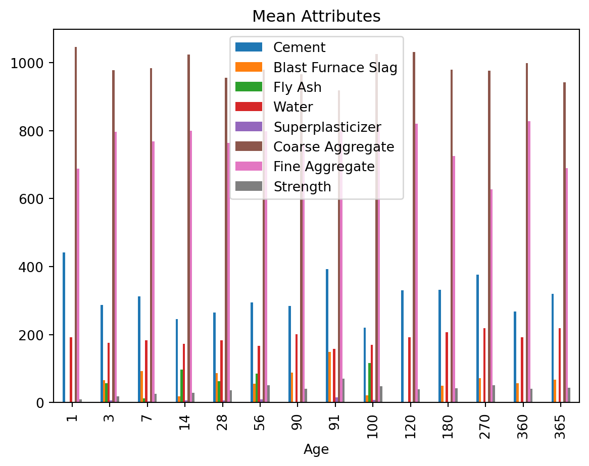
6.6 Analysis
Given the full data-set, we can compute the correlation between the columns given in the dataset.
correlation_data = data.corr(method='spearman')#correlation_dataimport seaborn as sns # seaborn is an alternative to Matplotlib with additional plotting options !
sns.heatmap(correlation_data)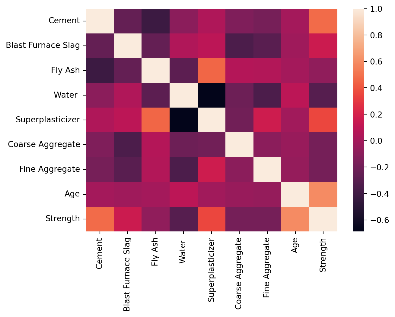
6.7 Data Cleaning
Not all datasets are clean due to several reasons, making data preprocessing a critical step in data analysis. Raw data often contains inconsistencies, errors, and missing values that can significantly impact the performance and accuracy of analytical models. Here are some reasons why datasets are often not clean and require preprocessing:
Data Collection Errors: During data collection, errors can occur due to manual entry mistakes, sensor malfunctions, or software bugs. These errors introduce inaccuracies and noise into the dataset.
Missing Values: Datasets frequently have missing values caused by incomplete data collection, errors in data storage, or non-responses in surveys. Handling these missing values is essential to ensure the dataset’s integrity.
Inconsistent Data Formats: Data collected from multiple sources may have varying formats, units, or scales. For example, dates might be recorded in different formats, or measurements could be in different units (e.g., meters vs. feet), necessitating standardization.
Outliers and Anomalies: Outliers can skew the results of data analysis and modeling. These extreme values may arise from measurement errors or genuine variations in the data, and identifying and handling them appropriately is crucial.
Duplicate Records: Duplicates can occur due to errors in data entry or merging multiple datasets. They inflate the dataset and can lead to biased or incorrect conclusions.
Noise and Irrelevant Data: Raw data often contains noise and irrelevant information that can obscure meaningful patterns. Filtering out this noise is necessary to enhance the signal-to-noise ratio in the dataset.
Data Imbalance: In classification problems, imbalanced datasets, where some classes are underrepresented, can lead to biased models that perform poorly on minority classes. Preprocessing steps such as resampling or generating synthetic data can help address this issue.
Inconsistent Data Entry: Human-entered data may have inconsistencies in spelling, abbreviations, or terminology. For instance, the same category might be labeled differently (e.g., “NYC” vs. “New York City”), requiring normalization.
Complex Data Structures: Datasets with nested or hierarchical structures, such as JSON or XML files, require flattening or transformation into a tabular format for analysis.
Preprocessing transforms raw data into a clean and usable format, addressing these issues through techniques such as data cleaning, normalization, transformation, and augmentation. This step is vital to ensure the quality and reliability of the subsequent data analysis or machine learning models, ultimately leading to more accurate and actionable insights.
Some of the important functions used for data cleaning using pandas are:
dropna(): This function is used to remove missing or null values from a DataFrame.

fillna(): This function is used to fill missing or null values in a DataFrame with a specified value or method.

replace(): This function is used to replace a specific value in a DataFrame with another value.

duplicated(): This function is used to check for and remove duplicated rows in a DataFrame.

drop_duplicates(): This function is used to remove duplicated rows from a DataFrame.

astype(): This function is used to convert the data type of a column in a DataFrame to another data type.

str.strip(): This function is used to remove leading and trailing whitespace from strings in a DataFrame.

str.lower(): This function is used to convert all strings in a DataFrame to lowercase.

str.upper(): This function is used to convert all strings in a DataFrame to uppercase.

rename(): This function is used to rename columns or indexes in a DataFrame.
The further options to clean data is discussed in this short subsection !
import pandas as pd
import numpy as np

# create a sample DataFrame
df = pd.DataFrame({'property': [100, 222, np.nan, 500, 500],
                   'info 1': [' velocity', 'distance   ', 'temperature ', 'weight', 'weight '],
                   'info 2': ['M/S', 'm', np.nan, 'KG', 'KG']})

print(df)
property info 1 info 2
0 100.0 velocity M/S
1 222.0 distance m
2 NaN temperature NaN
3 500.0 weight KG
4 500.0 weight KGThe next step is to clean the data by removing missing values:
# remove missing values
df = df.dropna()
print(df)
property info 1 info 2
0 100.0 velocity M/S
1 222.0 distance m
3 500.0 weight KG
4 500.0 weight KGNext we perform some basic data cleaning operations:
# remove leading and trailing whitespace from strings
df['info 1'] = df['info 1'].str.strip()
print(df)

# convert all strings to lowercase
df['info 2'] = df['info 2'].str.lower()
print(df)

# remove duplicates
df = df.drop_duplicates()
print(df)

# rename column names
df = df.rename(columns={'property': 'Value', 'info 1': 'Property', 'info 2': 'SI Units'})
print(df)
property info 1 info 2
0 100.0 velocity M/S
1 222.0 distance m
3 500.0 weight KG
4 500.0 weight KG
property info 1 info 2
0 100.0 velocity m/s
1 222.0 distance m
3 500.0 weight kg
4 500.0 weight kg
property info 1 info 2
0 100.0 velocity m/s
1 222.0 distance m
3 500.0 weight kg
Value Property SI Units
0 100.0 velocity m/s
1 222.0 distance m
3 500.0 weight kg6.7.1 Data import
However, most of the time, we already have data that is generated by another process and we need to import this data into a DataFrame !
Here’s a list of some commonly used functions in Pandas for reading data into a DataFrame:
read_csv: Reads a comma-separated values (CSV) file into a DataFrame. Can handle other delimiters as well.

read_excel: Reads an Excel file into a DataFrame.

read_json: Reads a JSON file into a DataFrame.

read_sql: Reads data from a SQL query or database table into a DataFrame.

read_html: Reads HTML tables into a list of DataFrame objects.

read_clipboard: Reads the contents of the clipboard into a DataFrame.

read_pickle: Reads a pickled object (serialized Python object) into a DataFrame.
These functions have various parameters to customize how data is read, such as specifying the file path or URL, specifying the delimiter or encoding, skipping rows or columns, and more. They also have several options to handle missing or malformed data.
6.7.1.1 Delimiter Options:
When reading data from a file, Pandas assumes that the values are separated by a comma by default. However, it provides various delimiter options to handle other separators such as tabs, semicolons, and pipes. Some of the delimiter-related options include:
delimiter or sep: Specifies the delimiter used in the file. For example, delimiter='\t' or sep='|' specifies tab-separated or pipe-separated values.

header: Specifies the row number(s) to use as the column names. By default, the first row is used as the column names.

skiprows: Specifies the number of rows to skip from the top of the file.

usecols: Specifies which columns to include in the DataFrame. It can be a list of column indices or names.
6.7.1.2 Encoding Options:
Data files may be encoded in various formats, such as ASCII, UTF-8, or UTF-16, and Pandas provides several encoding options to handle them. Some of the encoding-related options include:
encoding: Specifies the encoding of the file. For example, encoding='utf-8' or encoding='latin1'.

na_values: Specifies a list of values to consider as missing values. For example, na_values=['-', 'NA', 'null'].
na_values: This parameter allows you to specify a list of values that should be treated as missing or NaN values. For example, you might have a dataset where missing values are represented by the string ‘NA’. By passing na_values=[‘NA’] to the read_csv() method, Pandas will recognize this string as a missing value and replace it with a NaN value in the resulting DataFrame.
6.8 Exercises
6.8.1 Theory
- What is the difference between a Pandas Series and a DataFrame?
- How do you handle missing data in Pandas?
- What is the purpose of the groupby() function in Pandas?
- How do you merge two DataFrames in Pandas?
6.8.2 Coding
- Load the “iris” dataset from scikit-learn into a Pandas DataFrame. Then, group the data by the “species” column, and calculate the mean value of each column for each species.